Interpolation methods
If you have ever worked on a Computer Vision project, you might know that using augmentations to diversify the dataset is the best practice. However, some augmentations are not straightforward and built upon various mathematical concepts, for example, interpolation. On this page, we will:
Сover the general interpolation concept;
Draw a separating line between interpolation and extrapolation;
And check out such interpolation techniques as Nearest, Linear, Cubic, Area, and LANCZOS4.
Let’s jump in.
Interpolation method explained
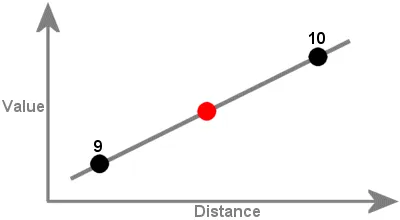
In maths, interpolation refers to finding a function’s value that exists within a sequence of data points. It can be described as the process of inserting an intermediate value between two other values.
For instance, in the example below, we can estimate the unknown value (red dot) based on the other known values (black dots).
Source
In the Computer Vision field in general and in image processing in particular, such a definition is also applicable. Let’s break down the interpolation concept and draw a simple example.
Suppose that you drew a beautiful painting and put it in a frame. At some point, you want to sell this painting, but your customers want it in a different size - say, some clients need a pocket-sized painting, while some prefer a painting covering the whole surface of their kitchen wall. To adjust to their needs, you need to resize your painting and change the frame as well. This is when you use interpolation.
Interpolation method Vs. Extrapolation method
The difference between interpolation and extrapolation in image processing is the following:
- Interpolation is used when we resize the image, which results in the image size changes. In Hasty, it is applied for Random sized crop, Resize, Shift Scale Rotate, Longest max size, and Smallest max size augmentations.
- Extrapolation is used when we rotate, downscale, or shift the image without changing its size. As a result of such transformations, some image parts are left empty, and extrapolation helps fill them in. In Hasty, it is applied for Shift Scale Rotate augmentation.
To draw an analogy with paintings, when you use interpolation, you change the painting’s size together with the frame, so there are no blank parts left between the image and the frame.
In comparison, you might rotate, downscale, or transform your painting without changing the frame. After that, some blank spaces might appear, and that’s when you use extrapolation to fill them in.
Both interpolation and extrapolation propose many various techniques, so let’s get straight into business and cover interpolation methods one by one.
Nearest interpolation explained
The Nearest algorithm takes the known value of the one nearest pixel without paying attention to other pixels.
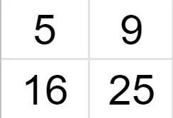
Suppose we have a 2x2 image and want to zoom it 2 times (so the size of the grid becomes 4x4).
Source
We know the values of some pixels, and now we have to interpolate the rest of the values.
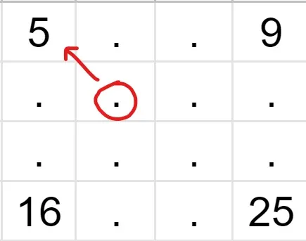
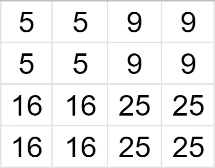
Let’s find the intensity of the pixel in the red circle. As you can see, its nearest neighbor with a known value is 5, so the value of the unknown pixel is also 5. In a similar fashion, we fill in the rest of the grid, and receive a 4x4 image.
Source
To reduce the image, we do a similar procedure. Suppose we have a 4x4 image and we want to shrink it 2 times, so the new grid is 2x2.
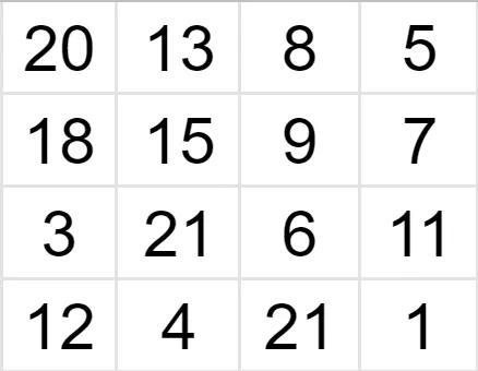
Source
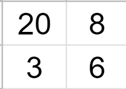
Since we are reducing our image by 2, we will drop out every second row and column of the image matrix.
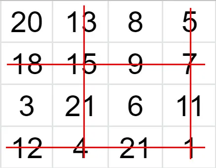
In the end, we are left with a 2x2 grid.
Source
As you see, the Nearest interpolation algorithm is the most straightforward to use. However, it might produce some distortions of the image due to its simplicity.
Linear interpolation explained
In Linear interpolation, we find the unknown value using the weighted average of its neighbors.
Let’s say we have a 1D row and want to expand it twice.
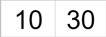
Source
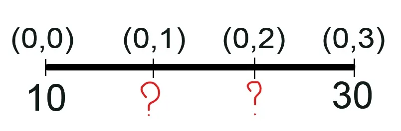
Source
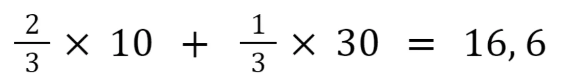
The following calculations are performed to find the second pixel:
And the third pixel:
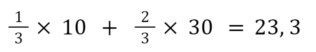
As you see, we assign different weights to the pixels with known values depending on their proximity to the pixel with the unknown value. The closer the pixel, the higher its weight in the equation.
In the case of 2D images, we apply the linear transformation both in the X and the Y directions, so both along the rows and the columns, in no particular order. Thus, this transformation is also known as bilinear interpolation. As a result of it, we use the weighted mean of the pixel’s 4 nearest neighbors (2x2 neighborhood) to find its value.
Linear (bilinear) interpolation slightly increases the computational burden but produces better results than the nearest-neighbor method.
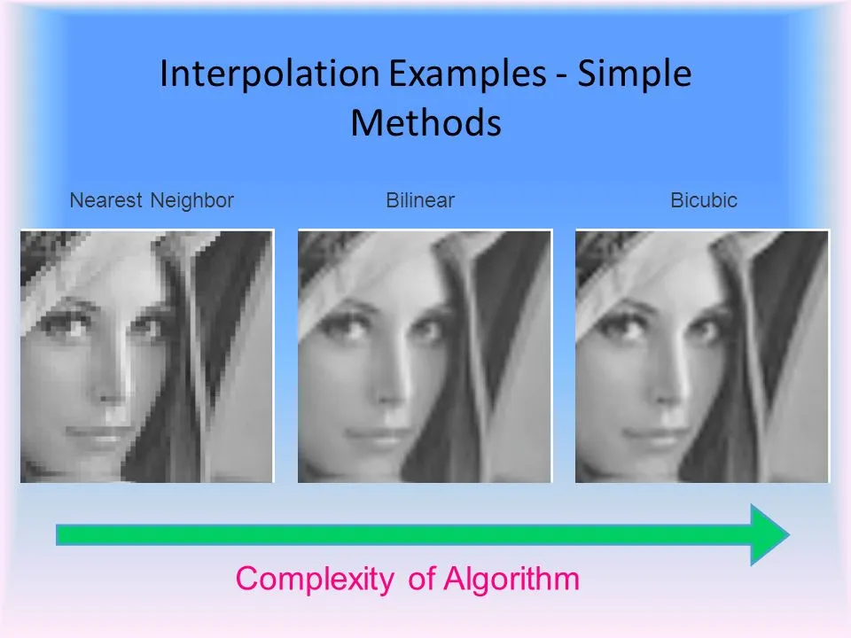
Cubic interpolation explained
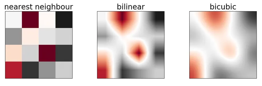
Cubic (or bicubic) interpolation is an even more refined algorithm that uses the 16 nearest neighbors (4x4 neighborhood) to calculate the unknown pixel’s value.
It preserves more details than the Nearest or Linear methods but also comes with a higher computational cost. Below you can see the comparison of the three methods.
Source
Source
Area interpolation explained
Area interpolation is commonly exploited in geographic research. This method uses the values of known geographical points to predict values of unknown points.
Area interpolation is widely applied to topographical, agricultural, hydrological, and other types of geographical spatial data. For example, if you need to shrink drone or satellite images, the Area interpolation technique might be useful for you.
LANCZOS4 interpolation explained
The LANCZOS4 interpolation uses the values of the 64 nearest pixels (8x8 neighborhood) to estimate the unknown value of the pixel.
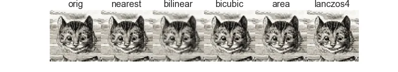
When to use which method
Generally, even though each case is unique, there are some observations that might be useful for you:
To shrink the image, it is best to use Area interpolation.
To zoom in on the image, it is best to use the Linear, Cubic, or LANCZOS4 interpolation methods (in the decreasing order of speed).
The Linear and the Cubic interpolations are slower than the Nearest and the Area interpolations.
The LANCZOS4 is the slowest algorithm.
Source

Source