Downsampling and Upsampling in Machine Learning
Computer Vision is impossible without image preprocessing. When researching the field, you might have encountered upsampling and downsampling terms. In vision AI, these are the names of techniques for rescaling images.
In everyday life, you probably come across the results of upsampling and downsampling applications daily: when surfing the web, viewing files, using image editors like Photoshop, zooming into some photos, etc.
On this page, we will:
Define the upsampling and downsampling terms;
See how upsampling and downsampling work;
Review some sampling algorithms;
Identify use cases and applications of upsampling and downsampling.
Let’s jump in.
What is image Downsampling?
Downsampling refers to a set of techniques that reduces the spatial resolution of an image while aiming to preserve its most valuable information.
For example, we might delete each 2nd row and column in the image, which will double down the image size. Thus, if the initial size were 1000x1000, the downsampled image would contain 500x500 pixels. However, as a human, you can still perceive what is portrayed in the downsampled image since we are usually very good at generalizing, recognizing patterns, and restoring information from context. For instance, if you watch a video on YouTube, you can still understand well what happens when you switch resolution from 480 to 360 and even to 240 pixels.
With that in mind, developers learned how to utilize the knowledge about the capacities and limitations of human perception to store and send information more efficiently with downsampling techniques.
What are the Downsampling benefits?
Downsampling provides the following advantages:
Image compression: downsampling decreases the size required for storing and transmitting the image;
Faster data processing: when you reduce the dimensionality of the images, they become faster to process.
What are the Downsampling applications?
Some typical examples of real-life use of downsampling include:
Web and mobile apps: whenever you open an image on the website, you want its preview to load as quickly as possible;
Real-time cases: object tracking, virtual reality, video streaming, etc;
Machine Learning enhancements: training CV models can go faster if you downsample the images in the dataset;
Artistic goals: one might want the image to appear smoother to hide some edges or sharp transitions in the image texture.
What are the Downsampling techniques?
Downsampling is a vast field. There are plenty of algorithms serving as a base for various downsampling techniques. Let’s cover the most popular ones.
Decimation
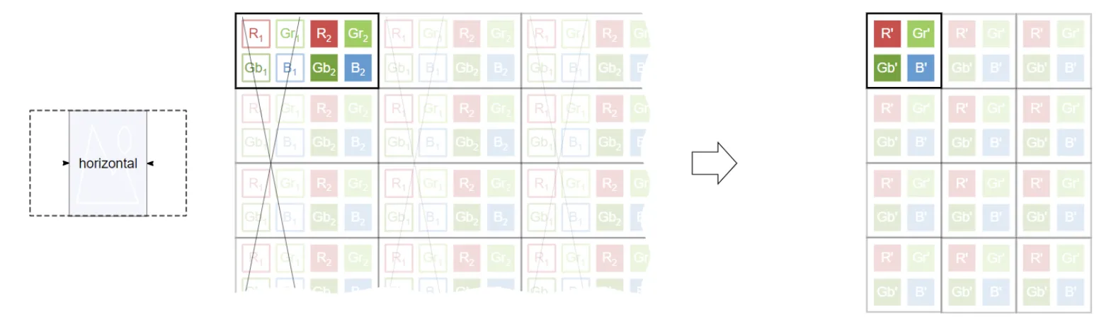
Decimation is a simple technique that decreases image resolution by skipping N pixels in rows, columns, or both columns and rows. You can tailor factors to your needs: for example, in a 2x1 decimation, you would skip every second pixel in a column and double down the image resolution. You can also choose combinations like 2x2 (this would reduce the resolution by a factor of 4), 1x4, 4x4, and so on.
If you work with colored images, you can also skip pixels pair-wise to preserve color.
Source
Mipmapping
The notion of mipmaps comes from computer graphics. To perform mipmapping, we take an original high-resolution image and create sequences of images, each representing the previous image in a lower resolution. Each “layer” is called a MIP* level and reflects different levels of details of the texture. Usually, each next image is scaled down by a factor of 2. For example, if the original input was 600x600, the second level will have a size of 300x300, the third one - 150x150, and so on.
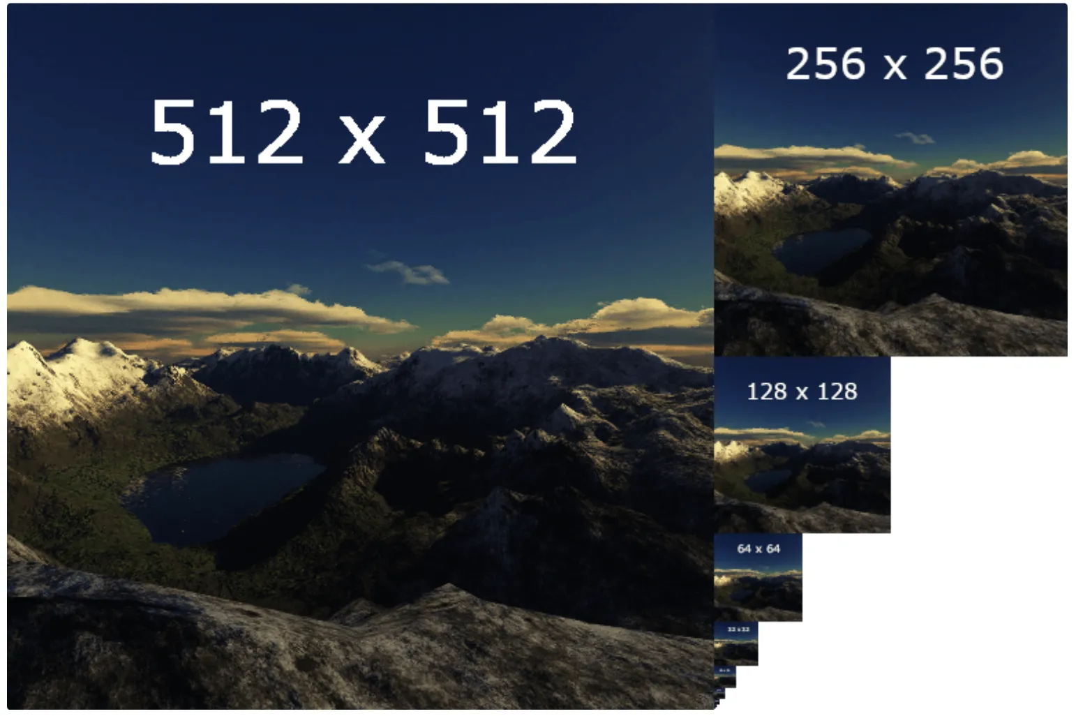
On the left is the original image, and on the right - the downsampled copies.
Source
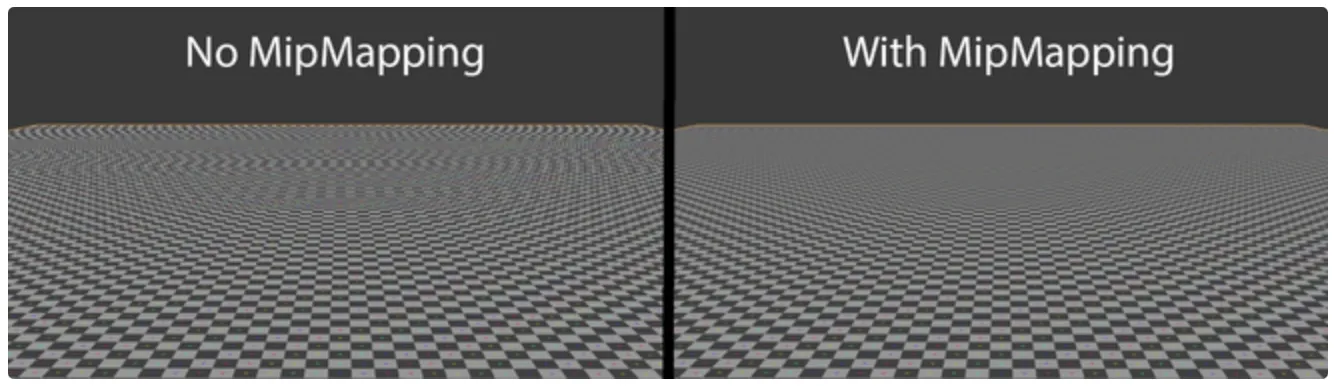
To understand the intuition behind this technique, imagine that each mipmap level reflects the distance from the camera to the texture. If the image is farther away, you will see a lower-resolution representation of it, and if it's closer to the camera, the representation will be high-resolution.
Source
Since mipmaps are pre-calculated, they require sufficient storage space. On the upside, they facilitate faster rendering, which is helpful in various fields, such as:
Map navigation;
3D Ccmputer games;
Virtual reality simulators;
Any other 3D applications.
Box Sampling
The box sampling algorithm maps the target pixel to a “box” of pixels on the original image and takes the average of the pixels inside the box as a new pixel value. Thus, all input pixels contribute to the output.
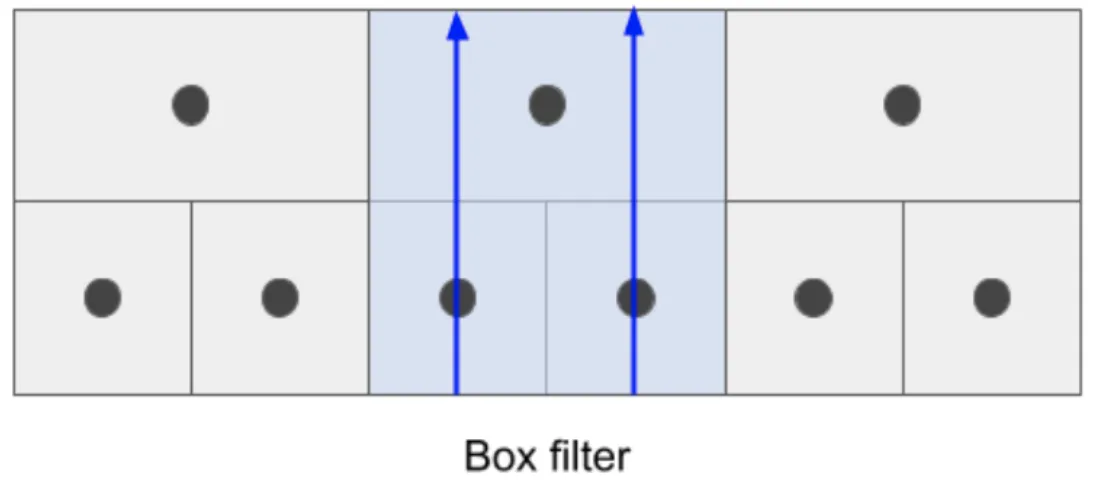
In this image, black dots represent pixel centers. The upper row is the low-resolution texture, and the bottom row is the original (higher-resolution) texture. Blue lines stand for the kernel's discretized weights.
Source
What is image Upsampling?
Upsampling refers to a set of techniques that increase the spatial resolution of an image. It is often used when you want to zoom in on some region in the lower-resolution image and avoid pixelation effects.
For example, if you have a 300x300 image and you want to show it on a display of 900x900 pixels, you would have to increase the number of rows/columns in the image and find a smart way to fill in the gaps. Of course, you could fill the missing values with zeroes, but that would give you just black spaces, and the image would not be perceived coherently. Hence, upsampling aims to find some way to construct a higher-resolution image that would be as close to ground truth as possible.
What are the Upsampling benefits?
The main advantage of upsampling is its ability to restore a higher-resolution version of the image without using any new external data but by utilizing the available data.
What are the Upsampling applications?
Some typical examples of real-life use of upsampling include:
Surveillance: often, the recordings from surveillance cameras are vague and low-quality, so it might be hard to distinguish people, objects, or numbers on the registration plates. Upsampling can make the image more сдуфк, to some extent;
Image editing: when the users zoom in on the image, you want to avoid them seeing pixels and noise;
Resizing the images: if you want to print the picture in a larger size, or insert a larger version of a low-resolution image into some web page, upsampling can help to resize the original image and minimize the loss in quality;
Medical imaging: medical images, like ultrasound of fMRI, might suffer from noise/pixelation due to restrictions in the equipment, the nature of the studied tissues, or some disturbances during the medical procedure itself. Enhancing image resolution can help to conduct thorough analyses and make diagnoses with more confidence;
Computer Vision: in encoder-decoder image segmentation models, we often downsample the input first to create lower-resolution feature mappings and later upsample them to get high-resolution feature maps. This step decreases computation costs and helps the model discriminate between classes more efficiently.
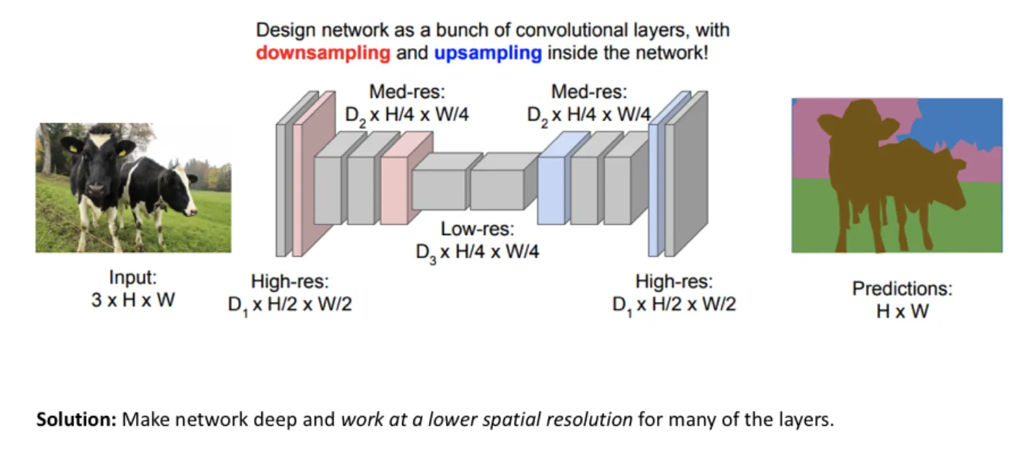
Source
What are the Upsampling techniques?
Upsampling is a vast field. There are plenty of algorithms serving as a base for various upsampling techniques. Mainly, the base algorithms are the different variations of interpolation.
Nearest Neighbor Interpolation
The Nearest Neighbor is the simplest type of interpolation. It takes the known value of the one nearest pixel without paying attention to other pixels.
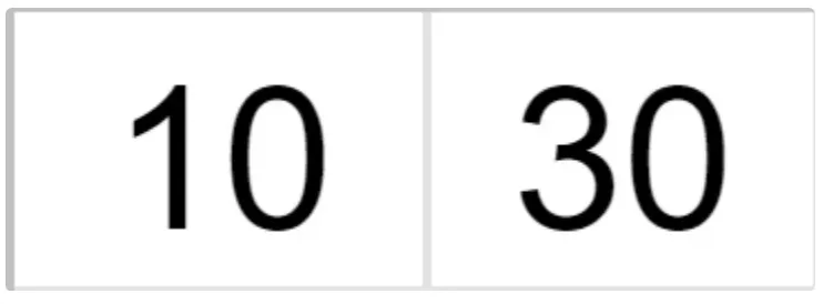
Suppose we have a 2x2 image and want to zoom it 2 times (so the grid size becomes 4x4).
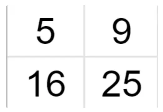
Source
We know the values of some pixels, and now we have to interpolate the rest of the values.
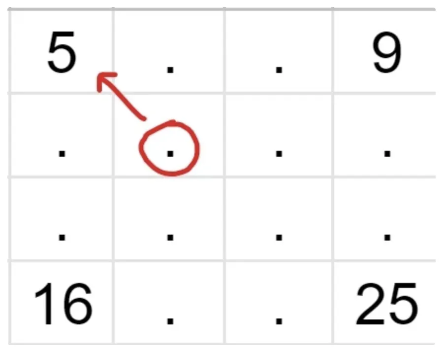
Source
Let’s find the intensity of the pixel in the red circle. As you can see, its nearest neighbor with a known value is 5, so the value of the unknown pixel is also 5. Similarly, we fill in the rest of the grid and receive a new 4x4 image.
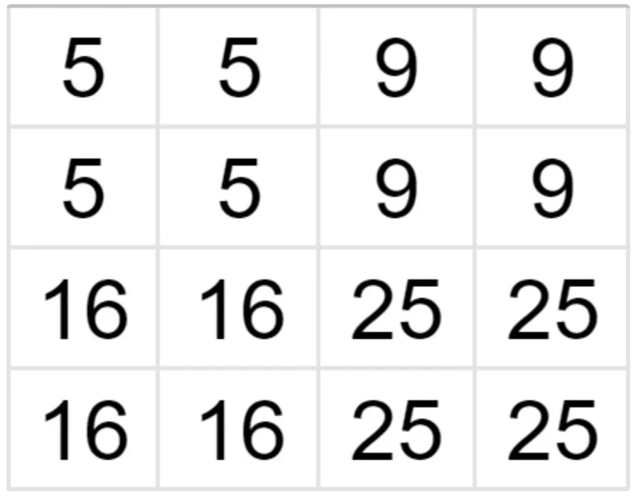
Source
Bilinear Interpolation
Bilinear interpolation is a more advanced technique that finds unknown pixel values by taking the weighted average of its neighbors. To explain how it works, let’s consider a simple 1D example of linear interpolation.
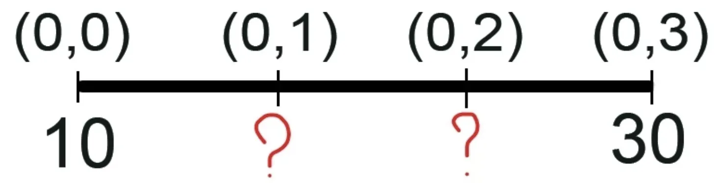
Say we have a 1D row (1x2) and want to expand it twice (1x4).
Source
Source
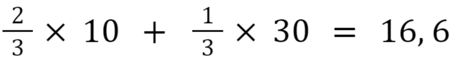
Let’s find the value of the first unknown pixel (0,1). It would be sensible to assume that the 0-th pixel affects it more, as it is its closest neighbor, while the pixel with coordinates (0,3) affects it too, though to a lesser extent. Therefore, we will assign the left known pixels a higher weight.
Source
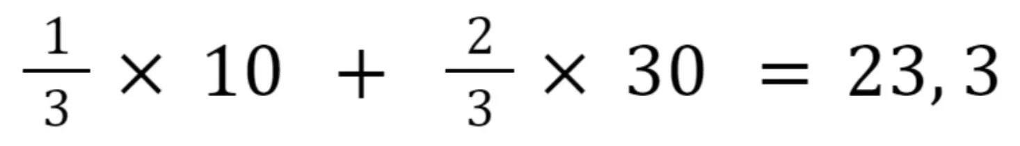
In a similar fashion, we assign weights for calculating the second unknown pixel.
Source
In the case of 2D images, we apply the linear transformation both in the X and the Y directions, so both along the rows and the columns, in no particular order. Thus, this transformation is also known as bilinear interpolation. As a result of it, we use the weighted mean of the pixel’s 4 nearest neighbors (2x2 neighborhood) to find its value.
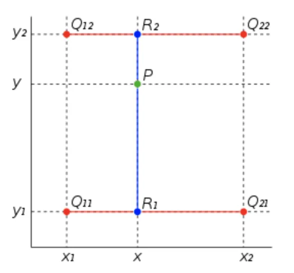
Source
For example, in the image above, to find the value of point P, we would have to:
Find the value of R1 by interpolating between known values Q11 and Q21 (x-axis).
Find the value of R2 by interpolating between known values Q12 and Q22 (x-axis).
Find the value of P by interpolating between R1 and R2 (y-axis).
Mathematically, it can be expressed as:
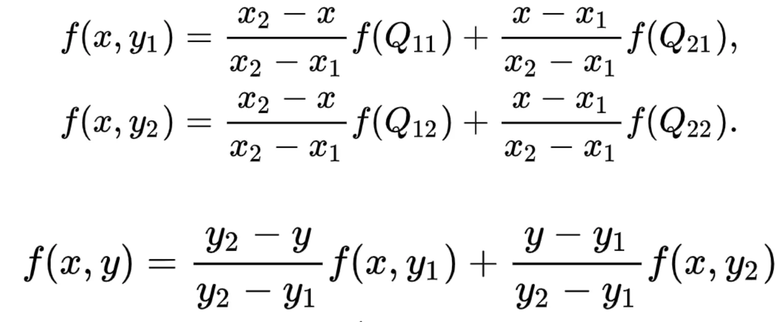
Source
Bicubic interpolation
Compared to Bilinear interpolation, which considers 4 nearest neighbors (an area of 2x2), Bicubic interpolation uses the 16 nearest neighbors (4x4 neighborhood) to calculate the unknown pixel’s value. Thus, it preserves more details than the Nearest Neighbor or Bilinear methods but also has a higher computational cost. If low computation time is not your top priority, Bicubic interpolation is the most advanced algorithm out of those described earlier.
Below, you can observe the comparison of the three methods in 1D and 2D. The black dot represents the point to be interpolated. As you can see, the Nearest Neighbor and Linear interpolations are more coarse and straightforward, while Cubic interpolation is more smooth and refined, as the curve gradient at each point depends on the 4 nearest points.
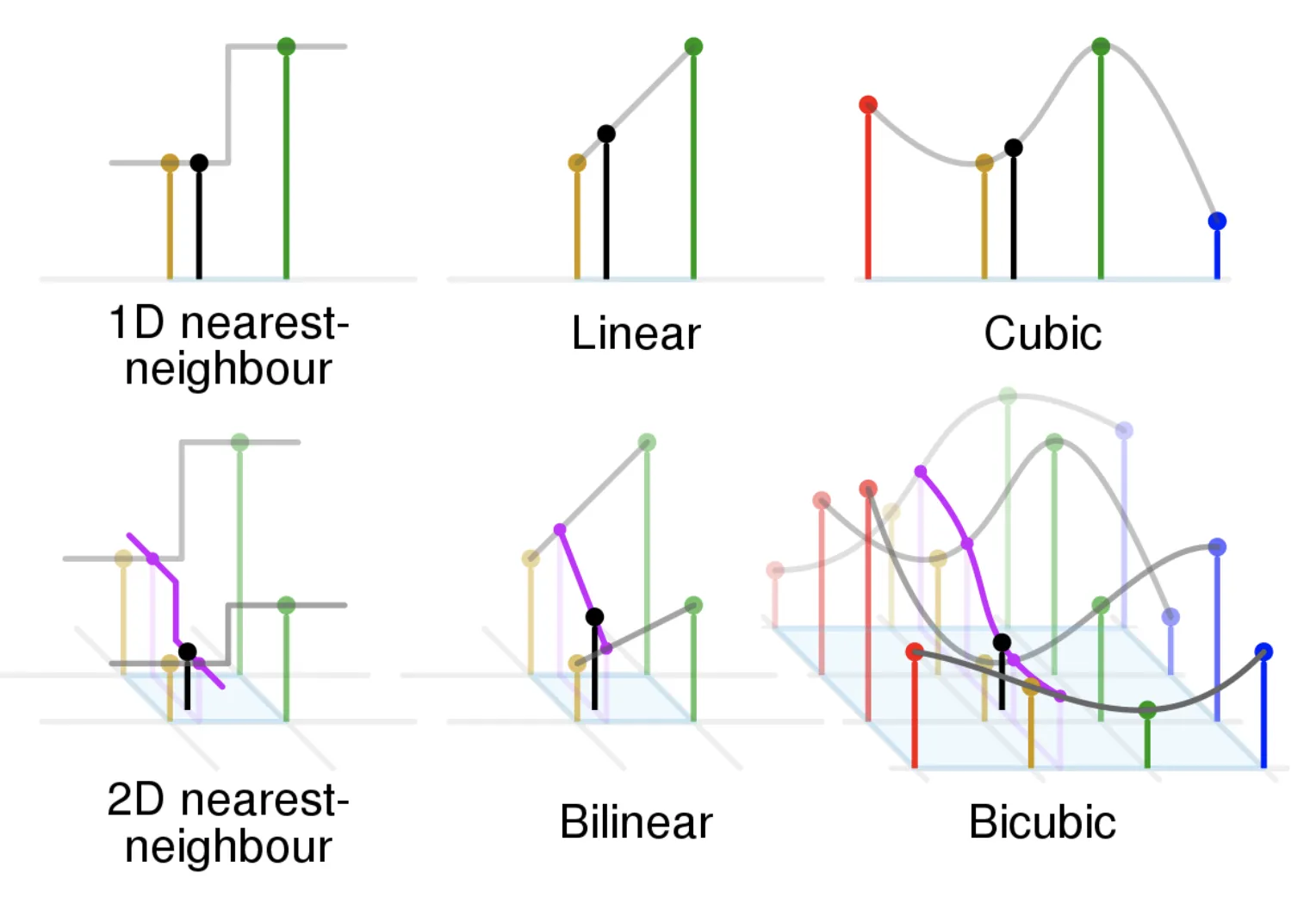
Source
The difference in the quality of the images upsampled with different techniques is quite visible.
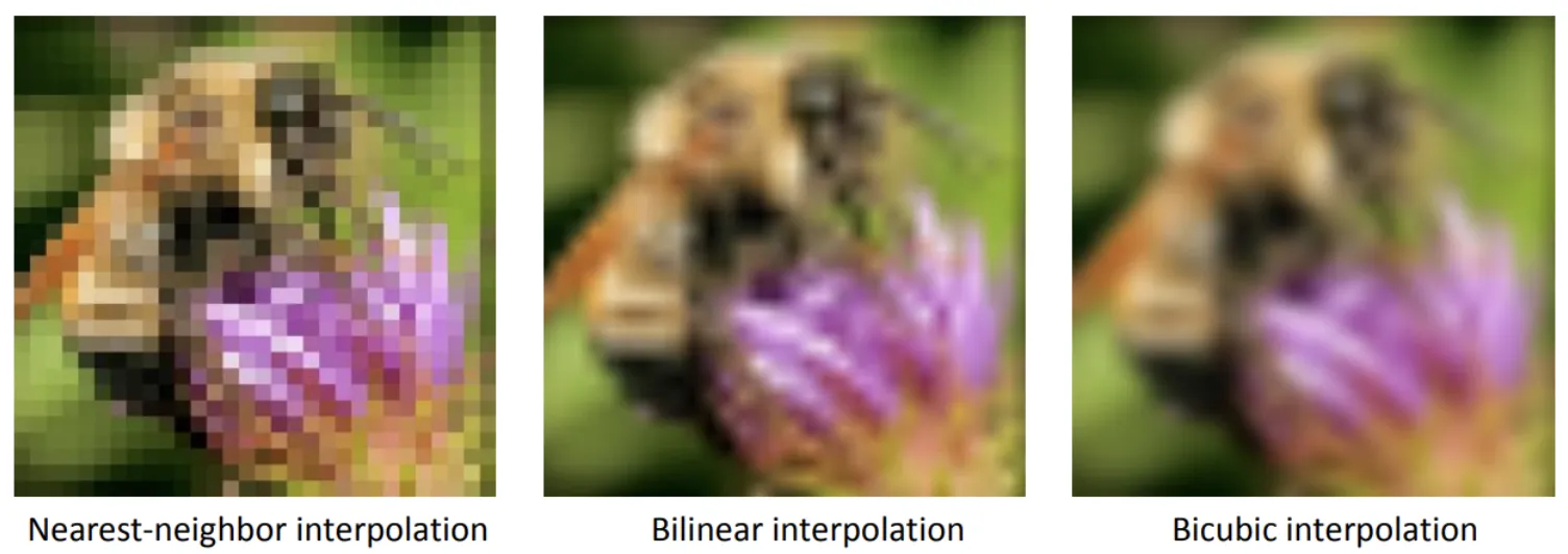
Comparison of the upsampled images' resolution
Source