Average Loss

Average Loss is a loss function available for Object Detection and Instance Segmentation tasks. If you select the average loss as one of the experiment parameters, you will see a graph at the end of the run that shows how the loss value changed during the training process.

How is Average Loss Calculated?

As the name suggests, the Average Loss function finds the average across different loss values of the model. In Hasty, we use the Average Loss for Object Detection and Instance Segmentation tasks, so let's peek into these two cases separately.

Average Loss for Object Detection

There are various architectures for Object Detection. The ones available in Hasty include the following:

• FBNetV3;

• Faster R-CNN;

• RetinaNet;

• CascadeRCNN.

All these architectures vary in their aspects. However, all Object Detectors follow two significant steps – classifying objects and detecting their bounding boxes. These can be referred to as Classification and Localization tasks.

Both classification and localization have their own loss functions.

• Regression loss stands for the loss calculated for the bounding boxes task;

• Classification loss stands for the loss calculated for the classification task.

Total Loss for Object Detection = Bounding Box Regression Loss + Classification Loss + (RPN localization loss)*

*RPN (Regional Proposal Network) Localization loss is specific to some models (like Faster R-CNN or Cascade R-CNN) and is, therefore, in parenthesis, denoting a particular case if a specific architecture is used. Different architectures used for the Object Detection task might affect the total loss differently.

To sum up, the algorithm for finding Average Loss in the Object Detection case is as follows:

1. Calculate the total loss for Object Detection for every batch;

2. Take the average across all the batches.

Average Loss for Instance Segmentation

Architectures for the Instance Segmentation task may also vary. In Hasty, you can find:

• Mask R-CNN;

• FBNetV3;

• CascadeMask R-CNN;

• HybridTaskCascade.

The loss for Instance Segmentation can be considered an extension of the Object Detection loss. This is because Instance Segmentation itself is partially built upon the Object Detection task.

In an IS task, we segment objects in an image. This gives us a more precise mask than the bounding boxes produced by OD. Each segment is a unique instance of a class.

Instance Segmentation also contains classification and localization tasks. Therefore, classification and regression losses appear in the equation. The only difference is that we add the mask loss that increases every time the model wrongly identifies the object's pixels.

Total Loss for Instance Segmetor = Mask Loss + Bounding Box Regression Loss + Classification Loss + (RPN localization loss)*

*RPN (Regional Proposal Network) Localization loss is specific to some architectures (like Mask R-CNN or CascadeMask R-CNN) and is, therefore, in parenthesis, denoting a special case if a certain architecture is used. Different architectures used for the Instance Segmentation task might affect the total loss differently.

The algorithm for finding Average Loss in Instanсe Segmentation is the same:

1. Calculate the total loss for Instance Segmentation for every batch;

2. Take the average across all the batches.

Interpreting the graph of Average Loss

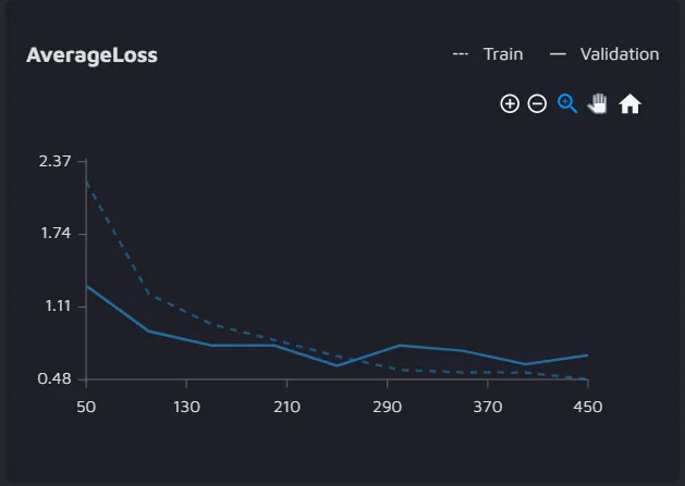
After running the experiment, you will likely end up with a graph for Average Loss that might look similar to the one below:

The graph displays the behavior of the Average Loss over the epochs during the training process.

In this graph:

• The x-axis represents epochs or iterations;

• The y-axis represents the Average Loss;

• The dotted line represents the performance on the training set;

• The solid line represents the performance on the validation set.

In our example, we see that the Average Loss for both train and validation sets shows a decreasing trend. This suggests that the model is learning and going in the correct direction minimizing the loss.

However, in some cases, you might see that the validation loss shows an increasing trend. Such a picture usually occurs when the model is overfitted and is too complex for the given dataset.

Fortunately, you can overcome overfitting by:

• Choosing a shallower network;

• Applying the early stopping technique by setting the patience parameter;

• Adding more diverse data to the dataset.

The training loss might also increase due to the underfitting of the model. Underfitting occurs when the model is too simple, which happens for different reasons – for example, you set too few parameters to describe the model.

In a broader sense, overfitting and underfitting occur due to the Bias-Variance tradeoff in Machine Learning.

Key takeaways

1. Average Loss is calculated by averaging the total loss over several batches in a dataset.

2. This total loss is different for Object Detection and Instance Segmentation tasks and depends on the architecture used for each task.

3. If the graph for Average Loss shows a decreasing trend for both training and validation datasets, then the model is going in the right direction.

4. If any of the curves in the graph shows an increasing trend, then it has to be fixed by tweaking the parameters while building the model.