PSPNet
Scene Parsing
Scene parsing is the process of segmenting and parsing an image into various visual areas that correspond to semantic categories such as sky, road, person, and bed.
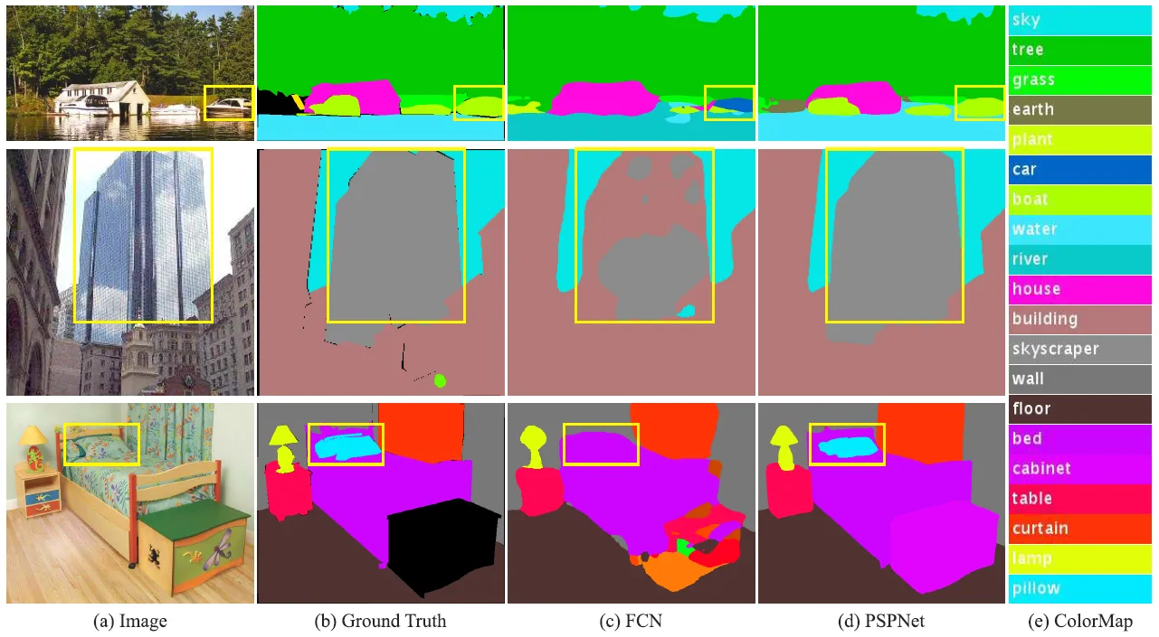
From the figure above we see that there are several issues with complex-scene parsing. The first row shows the issue of mismatched relationships – cars are seldom over water than boats. The second row shows confusion categories where the class “building” is easily confused with “skyscraper”. The third row illustrates inconspicuous classes. In terms of color and texture, the pillow in this case is extremely comparable to the bedsheet. These inconspicuous objects are easily misclassified by Fully Convolutional Network (FCN).
A deep network with a suitable global-scene-level prior can much improve the performance of scene parsing, and this is where PSPNet comes in, it is able to capture the context of the whole image to classify the object as a boat.
Pyramid Pooling Module
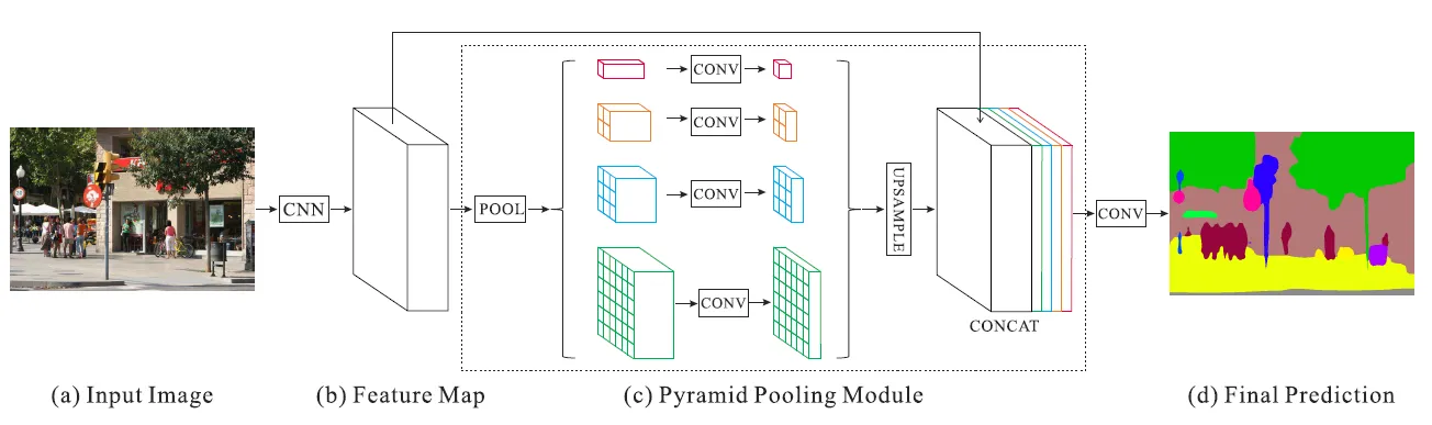
Given an input image, PSPNet uses a pre-trained ResNet model with the dilated network strategy to extract the feature map of the last convolutional layer. On top of this feature map, the pyramid pooling module is applied to harvest different sub-region representations. This is followed by upsampling on the pooled features to make them the same size as the original feature map. Afterward, these upsampled maps are concatenated with the original feature map to be passed to the decoder carrying both local and global context information which is fed into a convolution layer to get the final per-pixel prediction.
PSPnet in Model Playground
Encoder network
The PSPNet encoder contains the CNN backbone with dilated convolutions along with the pyramid pooling module. The use of the encoder network is to transform the raw input image into an intermediate input that is understandable by the neural network. For PSPnet, the feature map of the image is this intermediate input that is generated through a CNN backbone.
In Model Playground, several encoder architectures can be used to generate this feature map. They are:
- ResNet;
- EfficientNet;
- MobileNetV2;
- SWIN.
ResNet
ResNet is a feature extractor with very deep layers and skipped connections. The main idea behind ResNet is to build better models with increasing depth of the model by skipping the connections between some of the blocks.
For this encoder network, the depth of the ResNet and the weights can be selected.
Efficient Net
Efficient Net, an architecture that is searched using NARS (Neural Architecture Search), can also be used as a feature extractor.
Efficient Net subtype and the weights of the network can be chosen for this architecture.
MobileNetV2
MobileNetV2 was introduced as a new mobile architecture that improved the state-of-the-art performances of the mobile models. MobileNetV2 is based on depthwise separable convolution which is far more computationally efficient than the standard convolution. DSC (depthwise separable convolution) uses pointwise convolution of 1X1XM and depth-wise convolution of kXk on each of the channels of the filters.
This encoder is initialized with MobileNetV2ImageNet weights.
Users can also specify the width multiplier for this encoder network. The width multiplier is the factor by which the number of channels of the current layer is multiplied to obtain the number of channels in the next layer.
- If the width multiplier is greater than 1, then the number of channels will increase, and hence the number of different features also increases.
- If the width multiplier is less than 1, then the number of channels will decrease in every layer.
SWIN
SWIN is based on a transformer technology that is dominantly used for Natural Language Processing tasks. But SWIN is scalable when the input is an image and has outperformed the dominating CNNs in some scenarios.
- Size of the SWIN transformer: this parameter sets the size of the transformer that is used in the SWIN architecture. Larger the SWIN transformer later will be the vectors for the individual patches of the images that are used.
- Weights: this encoder network can be initialized with SWIN-T ImageNet weights.
- Window size: SWIN architecture uses shifted window-based self-attention. The attention spans a certain number of patches in the image. This is defined by the Window Size in the self-attention heads.
- Patch Norm: this determines whether to use the layer normalization in input layer patches.
- Absolute position Embeddings: position embedding is the process of adding vectors to individual vectors of input patches in order to encode their position in the image. Turning this on will use the absolute position encoding technique rather than the relative technique.
- Drop Rate: it is the rate of dropout used in the MLP inside the SWIN transformer. Like any other dropouts, this is used to regularize the model and prevent overfitting.
Advanced Options for SWINDrop path rate
- Drop path rate is the stochastic drop rate that aims to reduce the depth of the layer in the training phase of the network. This is achieved by dropping entire residual blocks and bypassing their transformations. The rate for this drop path can be set.
- Attention Drop rate: Self Attention is used in SWIN architecture. The attention drop rate is the dropout ratio of the attention weights.
- QKV bias: Query, Key, and Value are used in the attention mechanism. A learnable bias can be added to these values in the training process.
Weights
It's the weights to use for model initialization, and in Model Playground Random Initialization of weights is used.
Dropout
Dropout refers to randomly ignoring neurons making the network less sensitive to the specific weights of neurons, which in turn results in a network that is capable of better generalization and is less likely to overfit the training data. It is the probability of an element to be zeroed in the decoder output (right before the segmentation head)
In Model Playground PSPNet dropout can be set between 0 and 1.
PSP out-channels
In Model Playground the number of out-channels in the PSP decoder can be set with an increased number of output channels.