Comprehensive overview of loss functions in Machine Learning
In the Machine Learning field, the loss function (or cost function) refers to the difference between the ground truth output and the output predicted by the model. The bigger the difference - the higher the loss, or the punishment. Hence, during training, the goal is to find such model parameters (weights and biases) that minimize the loss and maximize the rate of correct predictions.
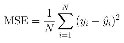
To illustrate the concept, let’s have a look at Mean Squared Error (MSE) - a classical loss function used in regression tasks, where both predictors and target variables are continuous (for example, predicting the house price based on its area). Its formula is given as follows:

Where:
N is the number of data points;
ŷ is the output predicted by the model;
y_i is the actual value of the data point.
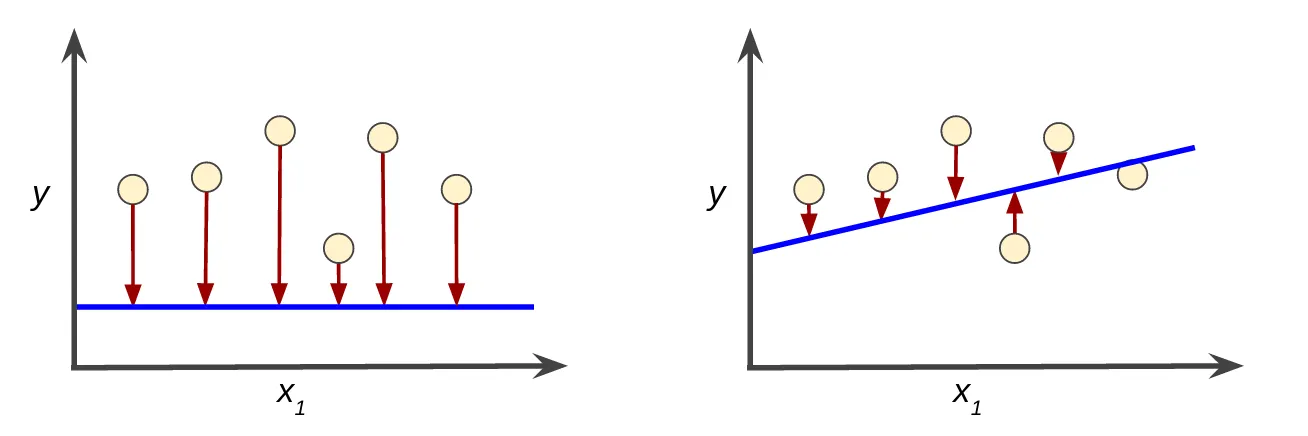
As you see, we simply sum the squared difference between each predicted and actual value and divide the result by the number of observations (data points). In the graphs below, the blue line represents the model’s predicted regression line, and the red arrows represent the error (loss) for each data point. It is visible with the unaided eye that the MSE will be notably smaller on the second graph.

Despite being common and easy to understand, the MSE loss function does not suit every use case for the following reasons:
It is sensitive to outliers: data points that greatly stand out from the rest may heavily influence the regression line, which leads to a decrease in model performance.
It does not work well with classification: MSE is used for regression tasks where the output is a continuous variable (unlike categorical variables like cat/dog/fish).
MSE tends to minimize large errors at the expense of the accuracy of smaller errors. As a result, the prediction line might be suboptimal.
In the next section, we will give you an overview of alternatives to MSE and briefly describe which loss function is suitable for a given Computer Vision (CV) task.
Overview of common loss function types in Computer Vision
- Cross-Entropy Loss is a widely used alternative for the MSE. It is often used for classification tasks, where the output can be represented as the probability value between 0 and 1. The cross-entropy loss compares the predicted Vs. true probability distributions. For example, if the animal in the image is a cat (cat = 1, dog = 0, fish = 0), and the model predicts the distribution as cat = 0.1, dog = 0.5, and fish = 0.4, the cross-entropy loss will be pretty high.
- Binary Cross-Entropy Loss is a special case of Cross-Entropy loss used. It can be utilized for any binary classification task and, in principle, for binary segmentation.
- Focal loss is used when class imbalance takes place in the dataset. In such cases, the model often learns to predict only the most represented class because, most of the time, the prediction will be correct, and the model will be rewarded. To prevent this, focal loss punishes the model more for wrong predictions on the "hard" samples (with the underrepresented class) and punishes it less on "easy" (more represented) samples.
- Bounding Box Regression Loss is used in object detection tasks to train models that predict the location of the bounding boxes for each object. This loss function is calculated by finding the difference between the predicted and ground truth bounding boxes.
- CrossEntropyIoULoss2D is a combination of the Bounding Box Regression loss and Cross-Entropy loss. In simple words, it is the average of the outputs of these two losses. It is often used for image segmentation tasks, where the ground truth is a pixel-precise mask of an object.
How to select loss function in Hasty
You can select the loss function during training before running an experiment.
- To start the experiment, first, access Model Playground in the menu on the left.
- Select the split on which you want to run an experiment or create a new split.
- Create a new experiment and choose the desired architecture and other parameters.
- Go to the Loss & metrics section and select the loss function. Since the choice of the loss function is heavily dependent on the task you are performing, sometimes only default options will be available to ensure smooth training.

