Advanced convolutional layers
When working on a Computer Vision (CV) project, the first thing one would want to know is probably the Convolution operation. With convolution being one of the basic CV concepts, understanding it is essential for exploring the vision AI field.
In this article, we will cover:
Parameters that deepen and expand the convolution concept;
Convolutional kernel;
Padding;
Stride;
Receptive field;
Different types of convolutions you might want to try out;
Transposed convolution;
Depthwise convolution;
Pointwise convolution;
Spatial separable convolution;
Depthwise separable convolution;
Useful techniques related to convolutions;
Blurring;
Edge detection;
Embossing;
And more.
Let’s jump in.
Convolution kernel
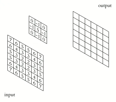
To put it simply, convolution is the process of sliding a matrix of weights over an image, multiplying every element piecewise, and then summing them to receive a new value of the new image. This window we move across the image is called the convolution kernel and is usually defined with the letter K.
Source
Performing the convolution operation reveals valuable features of an image, for example, edges, specific lines, color channel intensities, etc.
Source
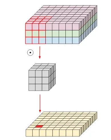
Convolution kernels are usually odd-numbered square matrices (usually but not necessarily!). One thing that defines a kernel is its size. Usually, kernels match the number of input channels, also called the depth.
If our input is a 32x32 colored image, then it has the dimension of 32x32x3 with a separate channel for each base color Red, Green, and Blue. Accordingly, our kernel would also have a depth of 3.
However, you can still tune the width and height of our kernel. You can go with a small window of size 3x3 or with a larger 5x5 or 7x7 (and beyond).
Intuitively, a small kernel size 3x3 will use only 9 pixels surrounding the target pixel to contribute to the output value, while larger kernels will cover more pixels. The logical question is how should I select the perfect kernel size. Unfortunately, there is no definite answer to that.
Still, it is good to know that:
Smaller kernels learn small features like edges well;
Larger kernels are better at learning the shapes of objects but are more affected by noise.
Moreover, if you opt for some well-known neural network architecture, you will not have to choose the kernel size, as the authors have already done it for you.
Blurring convolution
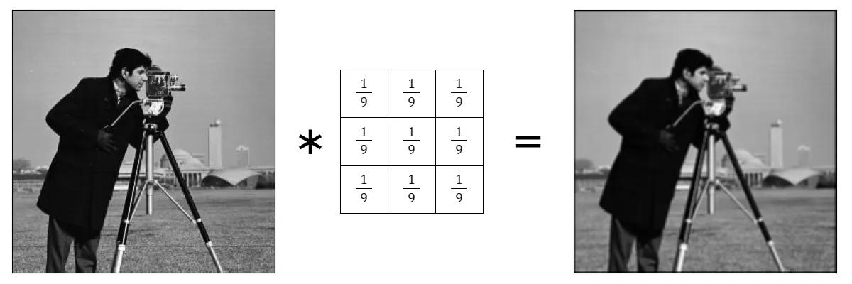
One of the uses of convolution operation is blurring images. Blurring an image means merging adjacent pixel values, making them less different from each other. There are various blurring techniques, but for simplicity, let's look at the most basic blurring with a mean filter.
Source
When you convolve an image with the kernel illustrated above, each output pixel will be the mean of 9 adjacent input pixels, resulting in a blurred image.
Edge detection convolution
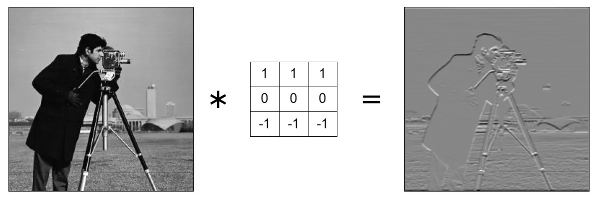
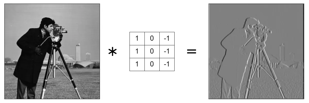
Another use for convolution operations is edge detection. In images, edges are sudden changes in pixel values. That being said, you can identify an edge by subtracting two-pixel values from each other. If the difference is large then it is an edge! Here you can see two examples of edge detection, horizontal edges detection, and vertical edges detection.
Source
Pay attention that you see only horizontal changes in pixel values. If you look closely, you can notice that the tall building behind completely vanished, because it has the shape of a strictly vertical rectangle.
Source
Here, on the other hand, you see vertical changes in pixel values, and the building is visible.
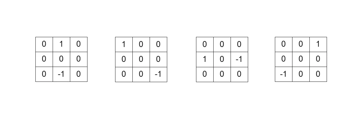
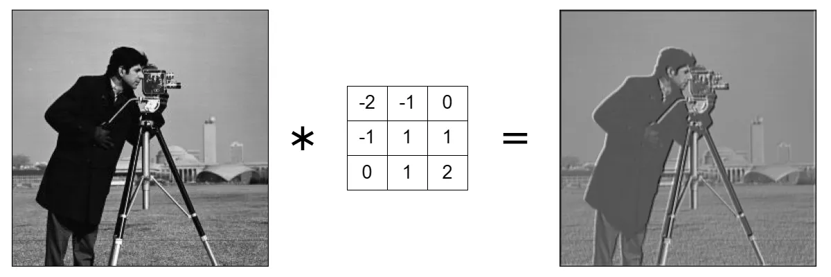
Emboss convolution kernels
Another type of valuable convolutional kernels are called emboss kernels. They are used to enhance the depth of the image using edges and highlights. There are in total 4 primary emboss filter masks. You can manipulate and combine them to enhance details from different directions to our needs.
Source
Source
Convolution parameter: Padding
We defined convolution as sliding a kernel across an input image to produce an output image. We can place the kernel so that its upper left corner matches the upper left corner of an image, but it would massively shrink the dimensions of the output feature map.
Let’s do something else and place the kernel so that its center matches the upper left corner of an image. Performing such a technique will mean that with every convolution, our image dimensions will shrink by (k-1) / 2 pixels, where k is the size of our square kernel.

The top left pixel of an image and a 3x3 convolution kernel. Red squares are values that are needed to compute a new value but do not exist.
Source
Let’s imagine you had an image of size 32x32 and applied the convolution with kernel 3x3. Then our output image has the dimensions of 30x30 because you had to ignore one line of pixels on every edge. To avoid that shrinkage of the dimension the padding concept comes into play.
Padding suggests filling the edges of an image with temporal values. Applying it lets you provide the missing values to compute an output properly. There are multiple ways of performing padding, so let’s closely examine them.
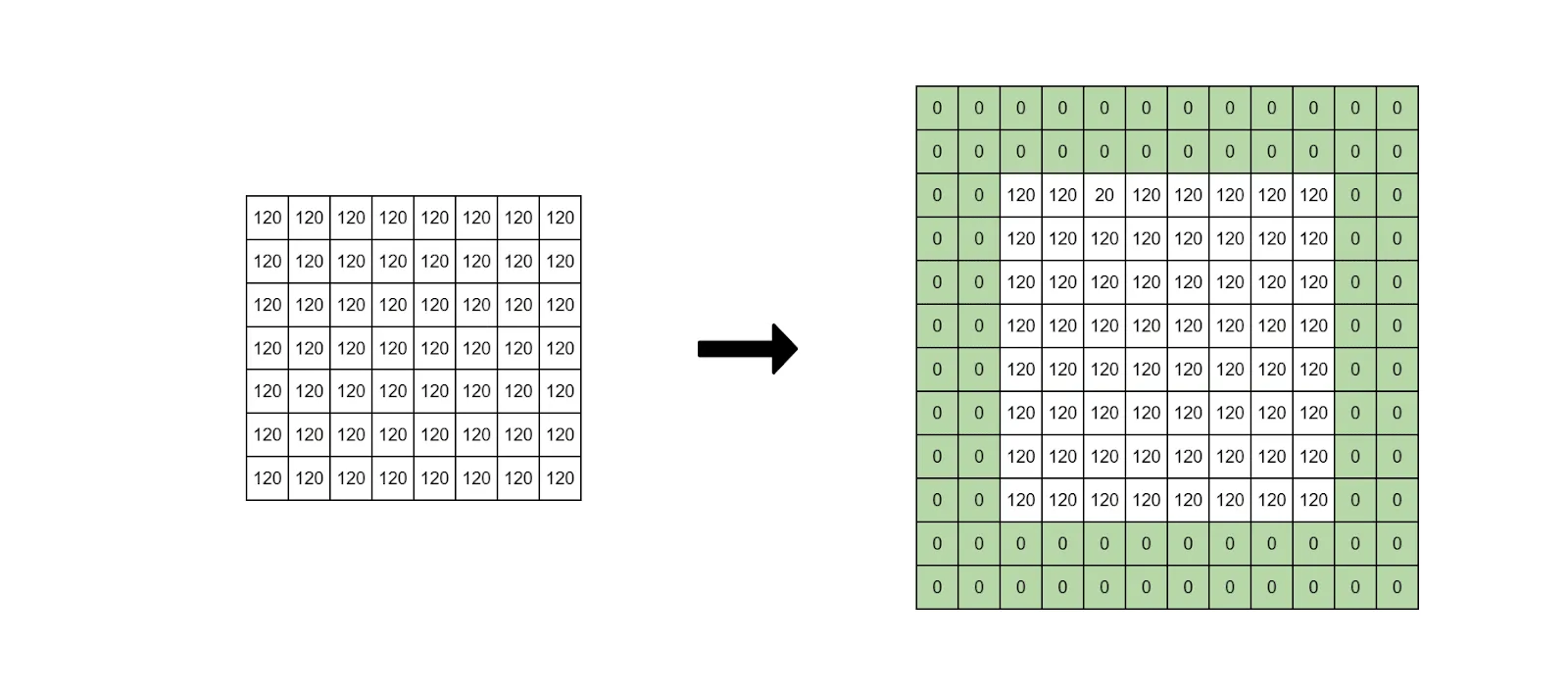
- Zero padding is one of the most simple and popular approaches. It works by simply adding zeros around an image.
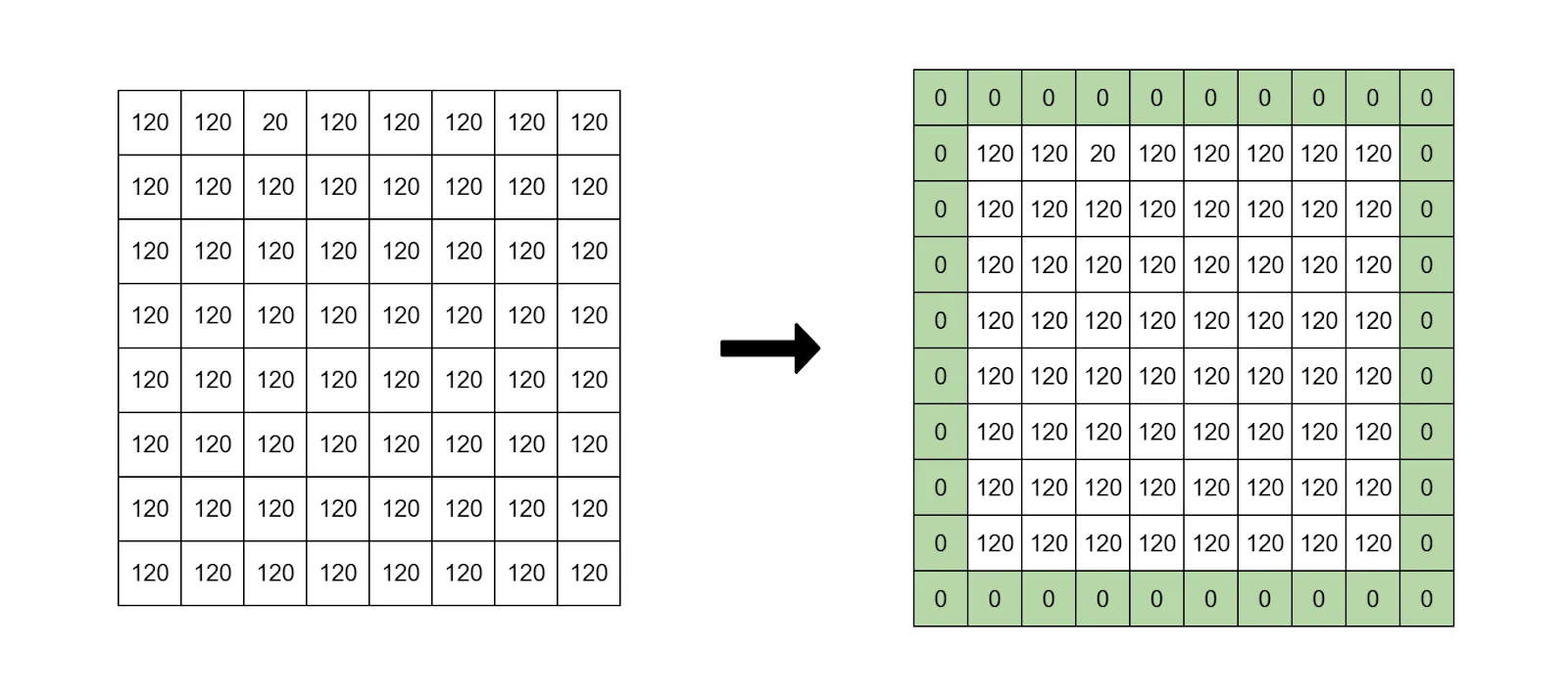
Green cells are temporarily added zero values.
Source
- Same padding is a padding that is set so the output dimensions after performing the convolution are the same as the input dimensions. If we input a 32x32 image and apply convolution, the output should have the same 32x32 size.
Source
- Reflective padding takes an edge pixel and uses its value as padding. This preserves the image structure on the edges and does not add non-existing values to it.
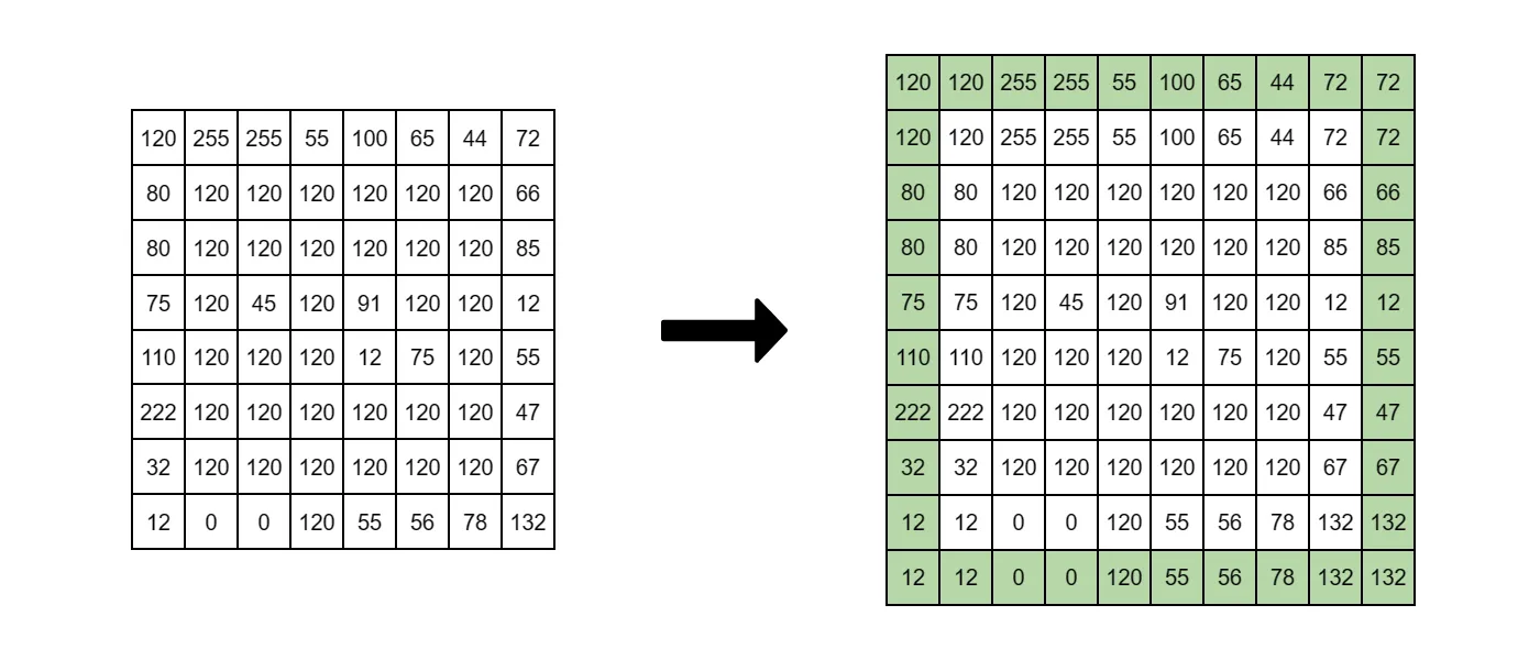
Source
Convolution parameter: Stride
Well, with padding, you can preserve the dimensions of the input. Now, let's talk about shifting the kernel across the image. The classic approach is shifting it 1 pixel at a time, but you can enhance the value. This is called stride.
Stride is the number of pixels the convolution kernel shifts across the image.
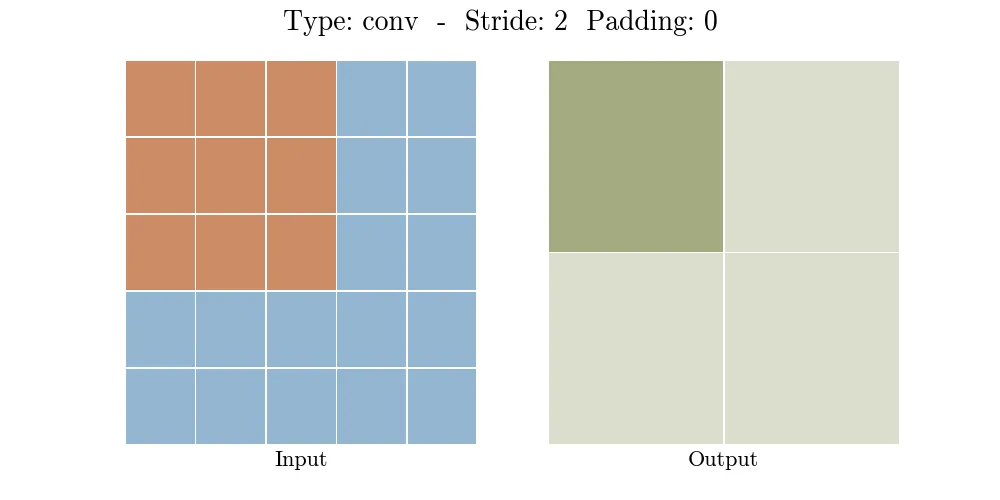
Left: Stride of 1
Right: Stride of 2
Source
But why don't we use larger strides? The simple answer is – they are not that effective.
One possible use case for a stride larger than 1 is when you have a huge input image and want to downsample it.
Setting stride to 2, in this case, reduces the image’s dimensions by half on the output, at the cost of losing valuable information.
Setting strides to larger values also reduces the computational load of the system, as now it does not perform convolution at every pixel. However, there are better ways for both performance optimization and dimensionality reduction, so the stride of 1 is almost always used.
How to calculate the size of the output feature matrix after the convolution operation?
So far, you learned that you could adjust your convolution operation by choosing the kernel size K, padding size P, and stride S. The big question is - how do you calculate the dimensions of the output matrix using all these numbers?
You can use the following formula:
where W and H are the width and height of the input image.
Let’s check out an example. Imagine having an input image of 9x9, a convolution kernel of 3x3, no padding, and a stride of 1. Then our output image dimensions are:
Let’s add padding to preserve the dimensions. Same example with padding of 1:
As you can see, adding padding preserved the initial size of the image.
Now, let's see how stride affects our output by increasing it to 2. Now the output dimensions are:
The size of the stride serves as the denominator for an image size. A stride size of 2 basically halves the image dimensions, and so on.
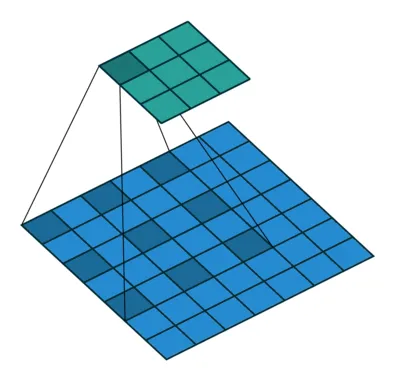
Convolution concept: Receptive field
If you use a kernel size of 3x3 then 9 pixels of the original image will contribute to a single pixel of the output image. That is called the receptive field of the pixel. It has a biological background. In biology, the reception field is the portion of the sensory space of our eyes that can trigger specific neurons in our brains. In computer vision, the receptive field has the same idea.
Source
If you chose a larger kernel size of 7x7, then the receptive field would also increase to 7 * 7 = 49, because now the output pixel value is affected by 49 input pixels.
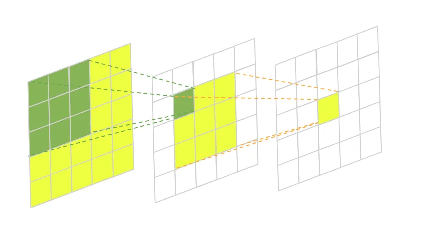
Now, imagine executing two consecutive convolution operations. Each uses a kernel of size 3x3. The receptive field of a pixel after the first operation is 9, that is simple. But the second convolution uses the output of the first convolutional operation as an input. That means that, although it also uses 9 pixels to produce a single output, each pixel it uses was made using 9 pixels of the original image. So, the receptive field of a pixel after the second convolution is 9 * 9 = 81 already.
What does the reception field tell us? The reception field of a pixel gives us an approximate idea of what this pixel represents. For example, a small receptive field of 9 might tell us that this pixel represents some edge or line on that area of the input image. But further into the model, the pixel can already represent some specific shape or a corner when the reception field increases.
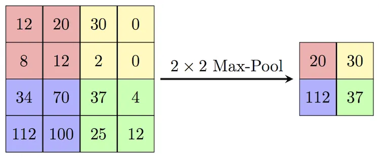
Pooling is a technique for downsampling an image. It takes several pixels and replaces them with one that represents them all. There are different types of pooling. Here are some of them:
- Mean pooling - take the mean of all pixels in the area;
- Max pooling - take the maximum value of the pixels in the area;
- Min pooling - take the minimum value of the pixels in the area.
Source
Pooling operation increases the reception field of the following convolutional layers by reducing the size of the output.
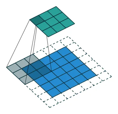
- Another method for increasing the reception field is dilated convolutions. It is easier to understand visually, so take a look at the animated illustration below.
Source
Source
Dilated convolution works by inserting holes (zero values) between kernel values to make it bigger. It was proven to improve the results of classification models.
Source
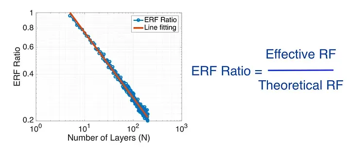
The Effective Receptive Field is the portion of the receptive field that has an actual influence on the output. If we have a kernel size of 3x3, then after 5 convolutional layers we would have a receptive field of 59049, but not all of these input pixels make an actual contribution to the output. Increasing the number of layers increases the theoretical receptive field, but the effective receptive field ratio decreases.
Transposed Convolution
You already know that the convolution operation reduces the dimensions of the input and that you can use padding to avoid that effect. But is there a way to get an increased dimension after the convolution? Yes, it turns out there is a special type of convolution called Transposed Convolution. It serves as a reverse operation for regular convolution. The produced output by this operation has a higher dimension than the input.
Transposed Convolution follows the following steps:
- Place s - 1 number of zeros between each pixel of input, where s is the stride of our regular convolution.
- Pad the resulting image with p zeros, where p is the padding size of our regular convolution
- Perform a regular convolution on the resulting input using a stride of 1.
Source
From the idea of transposed convolution, you can get the intuition that it is used for upsampling. Upsampling is the process of getting an image with a higher resolution than the input image.
This means that, for example, wyou feed 32x32 images into the convolution layer and get 64x64 images on the output.
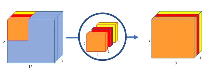
Depthwise Convolution
Next comes depthwise convolution. Remember that convolution kernels have the same depth as the input, and convolving with such kernels produces an output of depth 1? That is not the case for depthwise convolutions. Depthwise convolution applies different kernels of depth 1 to each input channel separately and then stacks results together again.
Source
Doing convolution in such a way always preserves the depth of the input. It will become clear why do you need it later, so for now stick to the definition.
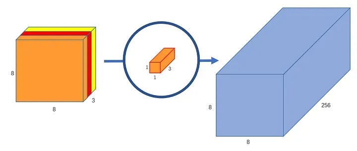
Pointwise Convolution
Pointwise convolution is somehow similar to depthwise convolution. In depthwise convolution you preserve the depth of our input, but change its width and height. In pointwise convolution we do the opposite.
Pointwise convolution uses a 1x1xN-sized kernel, where N is the depth of our input. If it has a stride of 1, then it always preserves the width and height of our input and does not need padding.
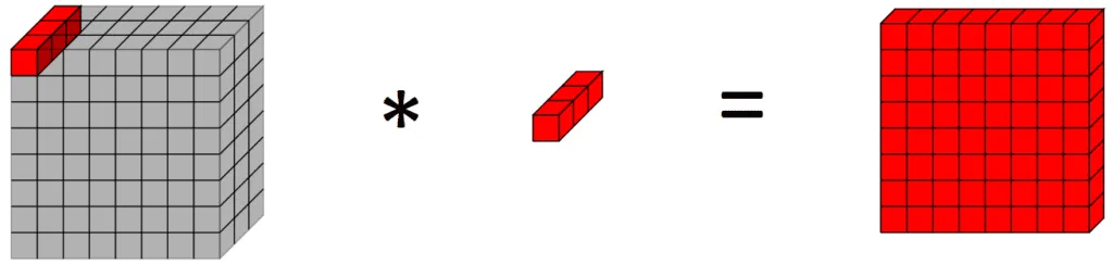
Source
Pointwise convolution observes only 1 pixel at a time and is used to regulate the feature channels. If you only want to increase the number of channels from 3 to 64, for example, without changing the input resolution, you can use 64 pointwise kernels and do it a lot more efficiently than the traditional convolution. However, in that case, these feature channels won’t learn much as they are guided by only a single pixel without a context. So it needed to be used in conjunction with something else.
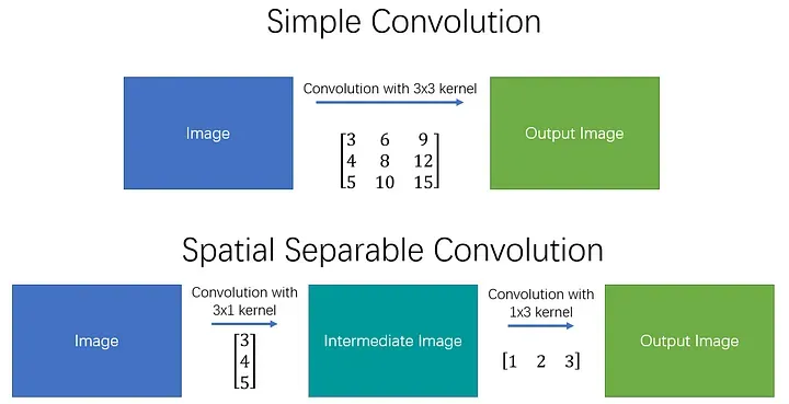
Spatial Separable Convolution
In real-life applications, a convolution operator is a lot “cheaper” than having a fully connected layer. However, there is a way to make it even more efficient, by introducing spatial separable convolutions. The mathematical concept of convolution allows us to separate our kernel into two linear kernels and apply them consequently to receive the same result.
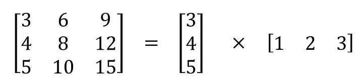
Source
This allows developers to perform convolution where instead of having to multiply 9 values and then add them up you can multiply 3 values 2 times and then add them up.
Source
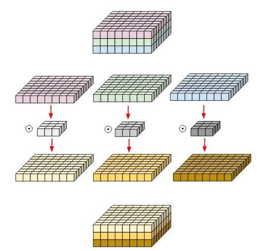
Depthwise Separable Convolution
Depthwise separable convolutions allow users to separate traditional convolutions into two operations even if the original kernel is not separable.
So how can you separate this pipeline into two separate more efficient operations? You already have the answer: you use depthwise and pointwise convolutions.
- First, you use depthwise convolutions to gather contextual data on the input, giving you some output of equal depth as the input.
Source
- And then you apply pointwise convolution with N kernels to this intermediate result to learn N feature channels.
Source
Performing these two operations separately is equivalent to the traditional convolution, but more efficient in terms of the number of computations, which makes it a popular choice for large CNNs where performance is crucial.