CyclicLR

If you have ever worked on a Computer Vision project, you might know that using a learning rate scheduler might significantly increase your model training performance. On this page, we will:

• Сover the Cyclic Learning Rate (CyclicLR) scheduler;
• Check out its parameters;
• See a potential effect from CyclicLR on a learning curve;
• And check out how to work with CyclicLR using Python and the PyTorch framework.

Let’s jump in.

CyclicLR explained

As you might know, many schedulers decrease the learning rate in a relatively monotonous manner. While this might be efficient in some cases, such methods have some drawbacks as well:

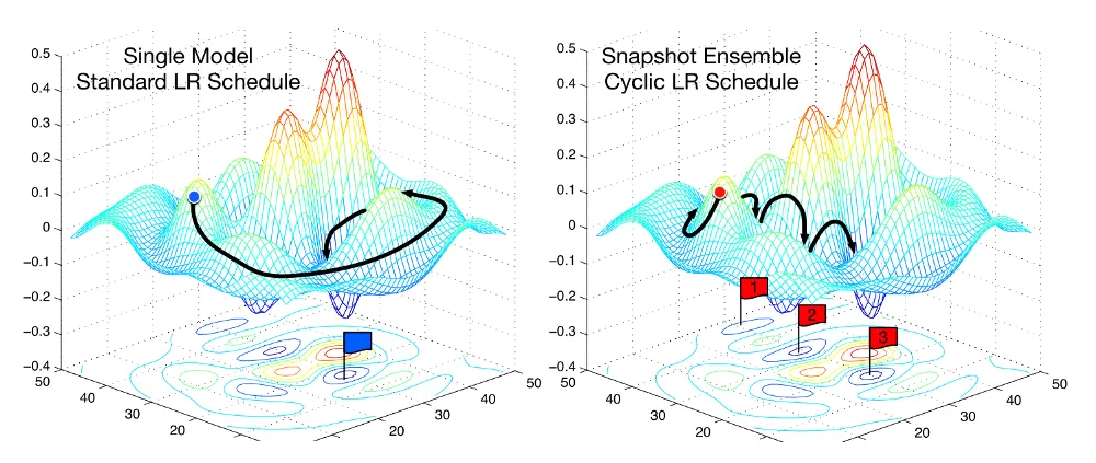
1. The model might get stuck in the local minima or a saddle point with a constant decrease in the learning rate. Since the learning rate values are decreasing only, it is hard for the model to break out from this “trap.”
2. The model’s success depends significantly on the initial choice of the learning rate. If it is set poorly, the model will likely get stuck soon, keeping the loss function high.

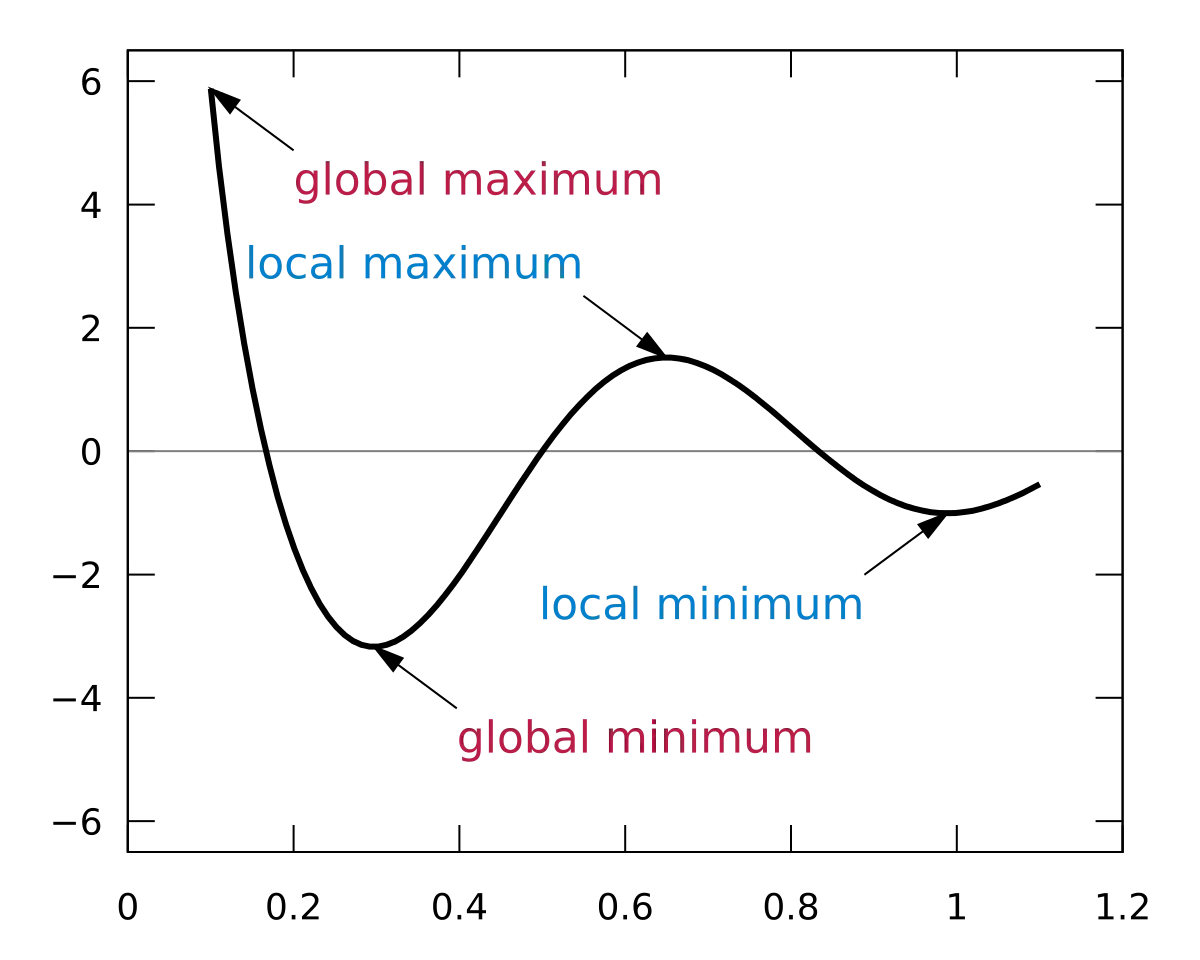
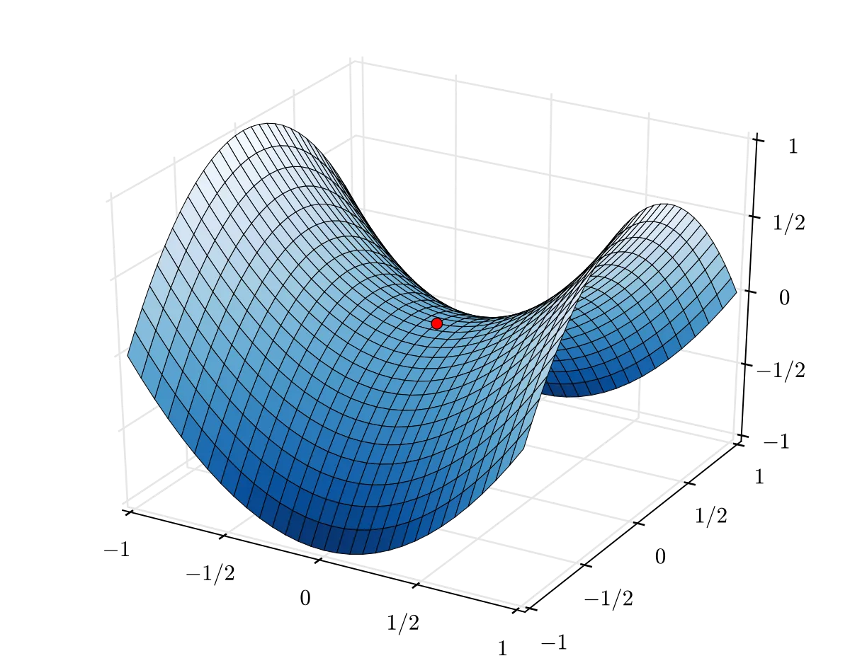
Cyclic Learning Rate is a scheduling technique that varies the learning rate between the minimal and maximal thresholds. The learning rate values change in a cycle from more minor to higher and vice versa. This method helps the model get out of the local minimum or a saddle point while not skipping the global minimum.

The general algorithm for CyclicLR is the following:

1. Set the minimum learning rate;
2. Set the maximum learning rate;
3. Let the learning rate fluctuate between the two thresholds in cycles.

Parameters

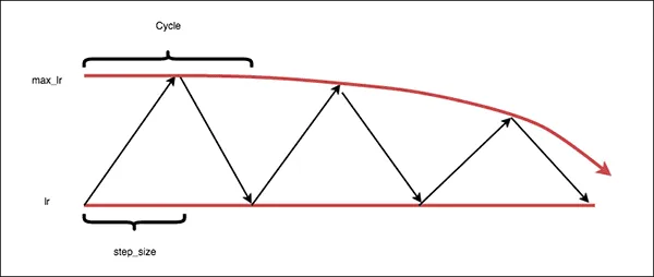
• Base LR - the initial learning rate, which is the lower boundary of the cycle.
• Max LR - the maximum learning rate, which is the higher boundary of the cycle.

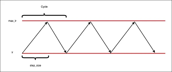
The step size reflects in how many epochs the learning rate will reach from one bound to the other.

• Step size up - the number of training iterations passed when increasing the learning rate from Base LR to Max LR.
• Step size down - the number of training iterations passed when decreasing the learning rate from Max LR to Base LR.

Mode - there are different techniques in which the learning rate can vary between the two boundaries:

• Triangular - in this method, we start training at the base learning rate and then increase it until the maximum learning rate is reached. After that, we decrease the learning rate back to the base value. Increasing and decreasing the learning rate from min to max and back take half a cycle each.

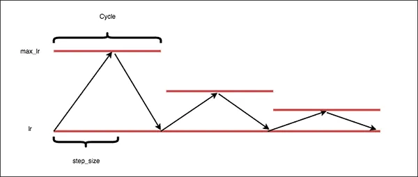
• Triangular2 - in this method, the maximal learning rate threshold is cut in half every cycle. Thus, you can avoid getting stuck in the local minima/saddle points while decreasing the learning rate.

• Exp_range - as well as the Triangular2, this method allows you to decrease the learning rate, but more gradually, aiming at exponential decay.

• Gamma - the constant variable in the ‘exp_range’ scaling function - a multiplicative factor by which the learning rate is decayed. For instance, if the learning rate is 1000 and gamma is 0.5, the new learning rate will be 1000 x 0.5 = 500.

• Scale mode - defines whether the scaling function is evaluated on cycle number or cycle iterations (training iterations since the start of the cycle):
  • Cycle;
  • Iterations.

• Base momentum - lower momentum boundaries in the cycle for each parameter group.

• Max momentum - upper momentum boundaries in the cycle for each parameter group. Functionally, it defines the cycle amplitude (max_momentum - base_momentum). The momentum at any cycle is the difference between max_momentum and some scaling of the amplitude; therefore, base_momentum may not actually be reached depending on the scaling function.

CyclicLR visualized

Code Implementation

      import torch
model = [Parameter(torch.randn(2, 2, requires_grad=True))]
optimizer = torch.optim.AdamW(model.parameters(), lr=learning_rate, weight_decay=0.01, amsgrad=False)
scheduler = torch.optim.lr_scheduler.CyclicLR(optimizer, base_lr, max_lr, 
step_size_up=2000, step_size_down=None, mode='triangular', gamma=1.0,cycle_momentum=false)

for epoch in range(20):
    for input, target in dataset:
        optimizer.zero_grad()
        output = model(input)
        loss = loss_fn(output, target)
        loss.backward()
        optimizer.step()
    scheduler.step()
    

Learn more about other schedulers…

• ExponentialLR;
• StepLR;
• MultiStepLR;
• ReduceLROnPlateau;
• CosineAnnealingLR.