Pooling
After grinding the convolution concept, the next logical step is to look closely at pooling in Machine Learning (ML) and Convolutional Neural Networks (CNNs). On this page, we will:
Check out the pooling definition in Machine Learning;
Understand why Data Scientists need pooling layers;
See the different variations of pooling layers;
Max Pooling;
Average Pooling;
Global Pooling;
Adaptive Pooling.
Check out the code implementation of pooling layers in PyTorch.
Let’s jump in
What is Machine Learning Pooling?
To define the term, in Machine Learning, pooling is a technique of reducing the spatial dimension of the data input while retaining its valuable features.
Pooling layers are most commonly used in CNNs in combination with convolutional layers. These two concepts perfectly fit one another, and they build the basis of the Feature Extractor for every CNN:
Convolutional layers extract essential information from the input data (images);
Pooling layers downsamples the spacial dimension of the output feature maps, thus reducing the algorithm’s computational complexity while retaining the valuable features extracted by convolutions.
Why are pooling layers needed?
If you are familiar with the padding concept, you might wonder whether pooling is needed. Yes, you can downsample input data through convolutional layers without adding additional actors, but pooling layers bring much more to the table.
Data Scientists use pooling for the following reasons:
- Downsampling is the core function of pooling. By reducing the input’s spatial dimension, you reduce the number of parameters and computation complexity of the whole network. Such an approach results in significant efficiency improvements and reduces the overfitting risks;
- The output feature maps you get after the convolution operation are location-dependent as they record the exact position of input features. Pooling addresses this challenge by making the network more robust to variations in the position, location, or scale of the features in the input data. This is called Translational Invariance. With pooling, the model will produce exactly the same response regardless of how the input is shifted. For example, you will get the same output for the input and horizontally flipped input.
- Usually, pooling layers care about the maximum and average values of specific regions of the output feature maps, thus identifying the most valuable features across the input.
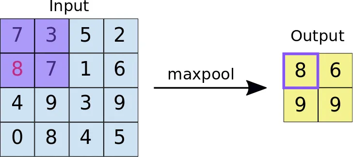
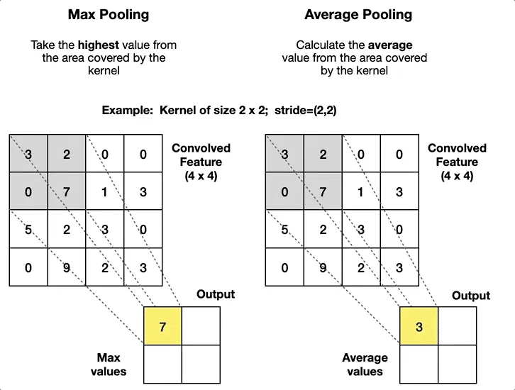
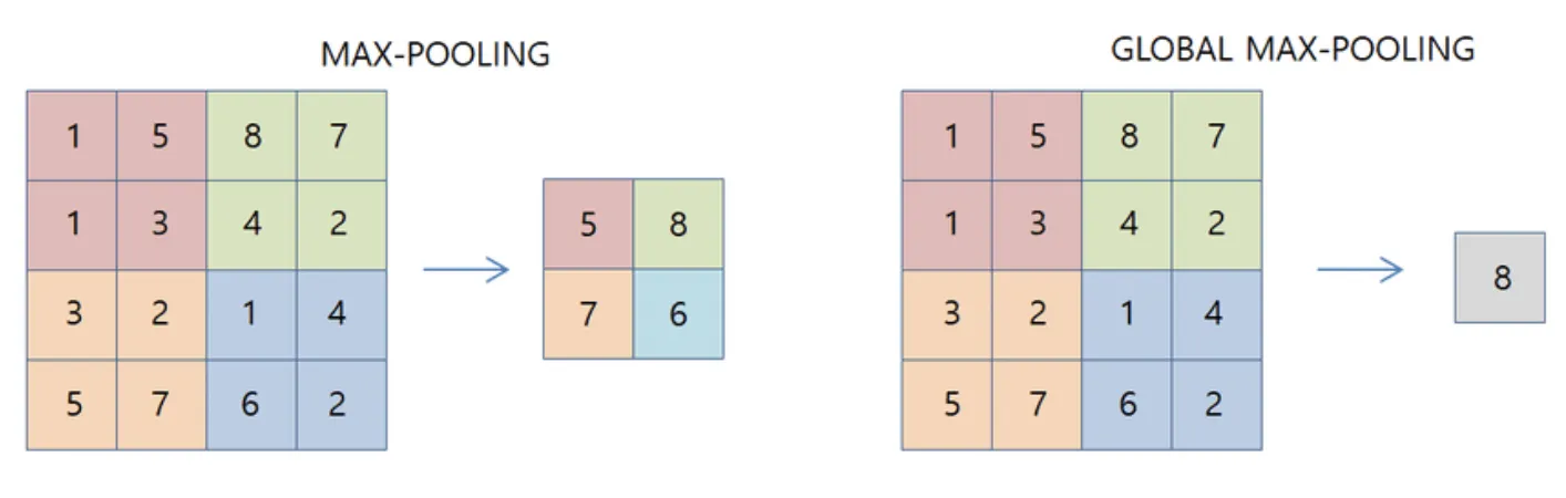
Max Pooling
Max Pooling is a pooling operation that finds the maximum value for every patch of a feature map and outputs it into a downsampled feature map. The algorithm for Max Pooling is as follows:
You initialize the kernel size for the pooling operation. This can be square or non-square;
You initialize other parameters that can influence the operation’s behavior, such as padding, stride step, dilation step, etc.;
The input is split into patches based on the specified parameters;
You go through each patch, select its maximum value, and output it to the downsampled map.
Source
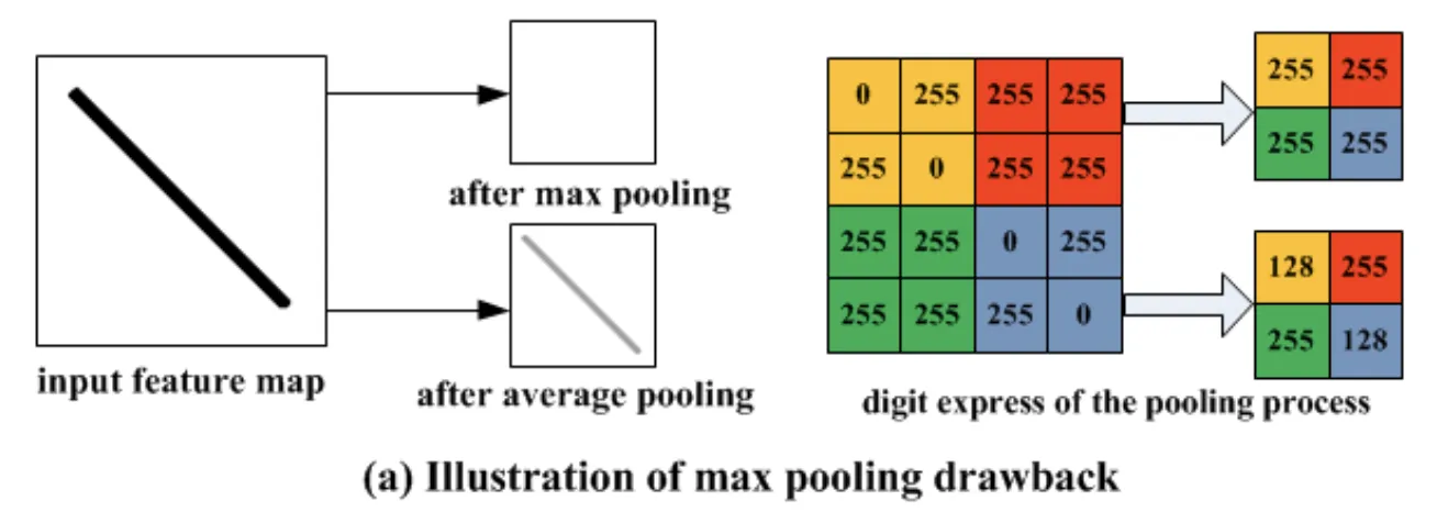
With its philosophy, Max Pooling preserves the most dominant features of the feature map and maintains some level of the input’s sharpness. However, this approach has a significant drawback of information loss.
As you can see, the Max Pooling technique completely ignores all the non-maximum values within each patch. This can lead to a significant loss of detailed information, which might cause problems in certain cases where details are crucial. For example, for segmentation and localization tasks, where precise spatial information is essential, max pooling may discard relevant information that could help accurately detect objects.
Source
Average Pooling
Average Pooling is a pooling operation that finds the average value for every patch of a feature map and outputs it into a downsampled feature map. The algorithm for Average Pooling is as follows:
You initialize the kernel size for the pooling operation. This can be square or non-square;
You initialize other parameters that can influence the operation’s behavior, such as padding, stride step, dilation step, etc.;
The input is split into patches based on the specified parameters;
You go through each patch, calculate the average value within the patch, and output it to the downsampled map.
Source
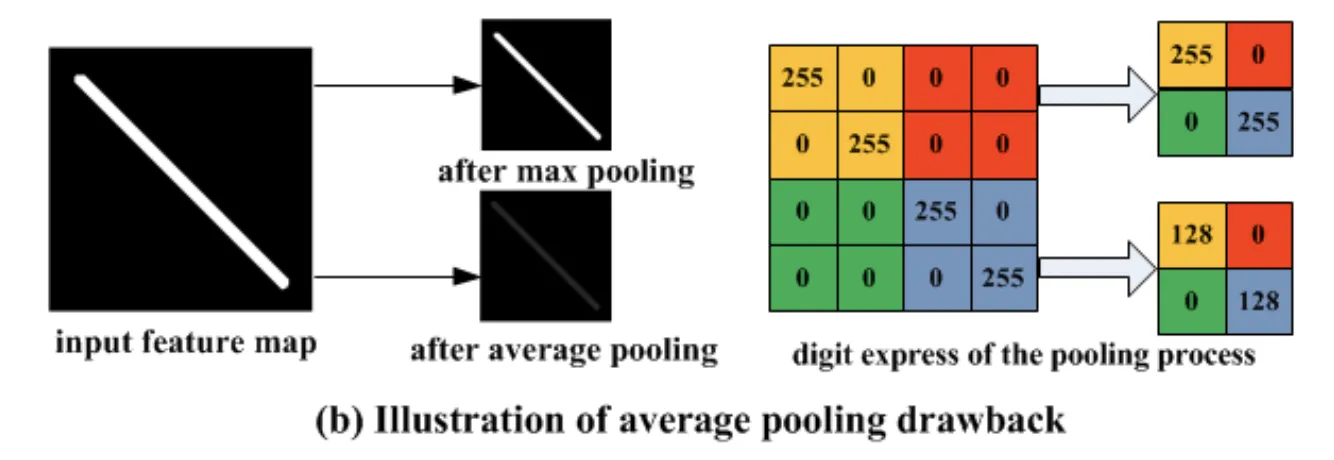
With its philosophy, Average Pooling blurs and smooths out the feature map’s details. You can view it from two different perspectives.
From one point of view, such an approach means that Average Pooling keeps the essence of features in the map and provides a balanced representation of the input. On the other hand, the smoothing effect results in a loss of sharpness, edges, etc. This might lead to a significant challenge for a model to capture objects' exact boundaries or spatial position.
Source
Global Pooling
The conventional neural network design approach suggests building a Feature Extractor (a combination of convolutional and pooling layers) and then passing the flattened representation of the output feature maps into a series of multilayer perceptrons that form the final output.
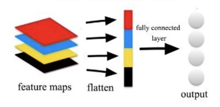
Simplified Convolutional Neural Network (CNN) structure
Source
However, if the end goal of the network is to obtain N values to feed an N-way softmax function to get the final probability vectors, there is an easier way to achieve this.
Design the Feature Extractor of the model in such a way that the final feature map has N channels (where N is the number of classes you want to predict) and apply one of the Global Pooling techniques to convert each channel into a single value.
So, Global Pooling techniques downsample the whole map instead of downsizing small patches and do not involve any learnable weights, which makes them computationally cheap compared to the traditional approach.
Global Average Pooling
Global Average Pooling suggests averaging each channel of the feature map to get N values as an output for an N-channel feature map.
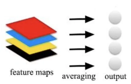
Source
Global Max Pooling
Global Max Pooling suggests taking the maximum value of each channel of the feature map so that you get N values as an output for an N-channel feature map.
Source
Adaptive Pooling
Some time ago, PyTorch introduced the Adaptive Pooling function. It comes in two versions - Adaptive Average Pooling and Adaptive Max Pooling. The idea of Adaptive Pooling is that a user does not need to define any hyperparameters except for the desired output size.
The function is designed in such a way that it would automatically calculate padding, stride, and kernel size to match the specified output dimensions. It might be pretty helpful if you decide to build a network’s architecture from scratch.
Pooling layer in Python
All the modern Deep Learning frameworks widely support pooling layers as they are the basis of the Feature Extractor of Convolutional Neural Networks. Therefore, all the options provided by TensorFlow, Keras, MxNet, PyTorch, etc., are valid, valuable, and worth your attention if you prefer a specific framework.