Comprehensive overview of solvers/optimizers in Deep Learning

In deep learning, the optimizer (also known as a solver) is an algorithm used to update the parameters (weights and biases) of the model. The goal of optimizers is to find such parameters with which the model will perform the best on a given task.

On this page, we will discuss:

• What is the idea behind solvers/optimizers, and how do they work;

• What are the main solvers/optimizers used in DL;

• What is the difference between a solver and optimizer;

• How to use solvers/optimizers in Hasty.

Let’s jump in.

Sovers/optimizers explained

As we mentioned in the intro, an optimizer is an algorithm that updates the model’s parameters (weights and biases) to minimize the loss function and lead the model to its best possible performance for the given task.

The loss function reflects the difference between the output predicted by the neural network and the actual ground-truth output. There are different types of loss functions; the final choice depends on the nature of your task and the data you work with. You can learn more about the Loss function on our MP Wiki page.

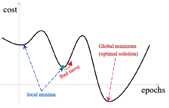
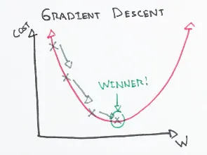
The most classical example of an optimizer is an algorithm called Gradient Descent (GD). It calculates the gradient (slope) of the loss function with respect to the weights and biases and updates them in the direction that minimizes the loss. The goal is to reach the global minimum (in comparison to local minima, as in the image below).

Generally, the formula for computing Gradient Descent is given as θ = θ - α∇J(θ), where:

• θ is the vector of parameters to be updated;

• α is the learning rate, which determines the step size at each iteration;

• ∇J(θ) is the gradient of the cost function J(θ) with respect to the parameters θ.

To give you more understanding of GD, let’s calculate one example manually. Say, we have to minimize a loss function defined as f(x) = x^2− 4x + 3.

Let’s initialize x_1 with the value 0, and set the step size (learning rate) as 0.3.

1. First, we should find the derivative of the loss function. In this case, it will be:
   f'(x) = 2x - 4
2. Then, we can plug in the x value:
   x_1 = 0
   f'(0) = -4
3. Now, we can update the parameters based on our learning rate and the gradient achieved with previous parameters:
   x_2 = x_1 - 0.3 * f'(x_1)
   x_2 = 0 - 0.3 * (-4) = 1.2
   As you see, our parameters shifted notably to the right, toward the global minimum (from 0 to 1.2).
4. Now, we take the updated parameters and plug them into the derivative again.x_2 = 1.2f'(1.2) = 2*1.2 - 4 = -1.6The loss value decreased from -4 to -1.6!
5. Again, we update the parameters.
   x3 = x2 - 0.3 * f'(x_2)
   x_3 = 1.2 - 0.3 * (-1.6) = 1.68
   

Steps 2 and 3 are repeated until the loss with the updated parameters actually stops decreasing. Of course, this fact alone does not guarantee that we found a global minimum; it could also be some local minimum. Various algorithms playing with the learning rate were developed to overcome this issue.

Even though Gradient Descent is relatively easy to comprehend and compute, it comes with its own disadvantages (that amplify as the dataset gets larger):

1. To calculate the gradient of the loss function, one should consider each training point from the dataset for each computation. This can lead to slow training and high computational costs.

2. Because the entire dataset is required for each computation, memory constraints might pose an issue.

3. When the dataset is large, there might be many local optima, and gradient descent may not converge to the global optimum. Hence, the model might underperform.

Overview of common optimizers in Computer Vision

There are other optimizers that address the shortcomings of Gradient Descent. Each of them has their own advantages and disadvantages, as well. Below, we will describe optimizers available to you in Hasty.

• Stochastic Gradient Descent (SGD), for example, is a variant of GD that computes the gradient on a random small batch of training data (so-called “mini-batch”). This can lead to faster convergence and better usage of memory. It is a preferable choice to GD when you work with large datasets.
• Adagrad (Adaptive Gradient) optimizer is worth considering if you work with sparse data, especially in high dimensions. The learning rate for each parameter is adjusted based on its gradient history. Nevertheless, Adagrad's learning rate may decrease too quickly, which could result in slow or too early convergence.
• Adadelta addresses the decaying learning rate problem found in Adagrad. The difference is that Adagrad considers all the past gradients to make an update, whereas Adadelta takes only a certain range of past gradients into the calculation.
• ASGD (Average Stochastic Gradient Descent) averages the weights that are calculated in every iteration. This makes it potentially suitable for cases when the dataset is large and noisy/has high variance.
• Rprop (Resilient Backpropagation) updates the learning rate for each weight separately based on the sign of the weight gradient. This helps the model converge faster and avoid oscillations. The performance of Rprop is better on noisy/highly variable or sparse data.
• RMSprop (Root Mean Square Propagation) also uses different learning rates for each parameter. The update of the learning rate is based on the root mean square of the weight gradients.
• Adam (Adaptive Moment Estimation) is one of the most popular and best-performing optimizers in the field of Computer Vision. It extends Stochastic GD with adaptive learning rates, like in RMSprop. If you want fast training with good accuracy, this might be your way to go.
• AdaMax can be viewed as an extension of Adam. It updates weights inversely proportional to the scaled L2 norm (squared) of past gradients.
• AdamW differs from Adam in that it regularizes the weight decay to prevent overfitting. Hence, AdamW tends to generalize a bit better.
• Lion (EvoLved Sign Momentum) is a relatively new but promising optimizer proposed in a research paper in 2023. It aims to address the limitations of traditional optimization algorithms such as Stochastic Gradient Descent (SGD) and AdamW.

To sum up, the choice of the optimizer depends on various factors:

• the task you are performing;
• the size of the dataset;
• the variance of your data;
• the complexity of the model;
• etc.

Difference between Schedulers and Optimizers

While both schedulers and optimizers aim at improving the model’s performance, these are two different types of algorithms.

• Optimizers adjust the weights of the neural network during training with the goal of minimizing the loss function. They work by computing the gradient of the loss with respect to the weights and then updating the weights in a way that reduces the loss. Examples of optimizers include Gradient Descent, Stochastic Gradient Descent, Adagrad, RMSprop, Adam, and so on.
• Schedulers adjust the learning rate during training in order to improve the performance of the optimizer. They work by reducing the learning rate as the training progresses, which can help the optimizer converge more efficiently and avoid getting stuck in local minima. Examples of schedulers include StepLR, MultiStepLR, CyclicLR, ExponentialLR, ReduceLROnPlateau, CosineAnnealingLR, and so on.

In other words, optimizers are responsible for updating the weights of the neural network to minimize the loss, while schedulers are responsible for adjusting the learning rate used by the optimizer to improve convergence and performance.

How to use solvers/optimizers in Hasty

Solvers/optimizers are used during model training and running the experiments.

1. To start the experiment, first, access Model Playground in the menu on the left.
2. Select the split on which you want to run an experiment or create a new split.
3. Create a new experiment and choose the desired architecture and other parameters.
4. Go to the Solver & scheduler section and select the solver you want to use.
5. Select solver parameters. They might differ from solver to solver, but the most common ones are:
   1. Base learning rate;
   2. Weight decay.